Many practitioners have been taught to describe a process using sigma levels. Yet these levels are commonly misinterpreted. This article will help you to understand the problem and learn more appropriate ways of describing your process.

In the days before handheld calculators and personal computers, students in SPC classes were taught to estimate the fraction of nonconforming product by converting each specification limit into a z-score and then looking up the fraction nonconforming using a standard normal distribution. Since the normal is the distribution of maximum entropy, this approach would, in most cases, yield worst-case estimates for the fraction nonconforming. Figure 1 shows these traditional fractions nonconforming for symmetric specifications spaced at different distances from the mean.

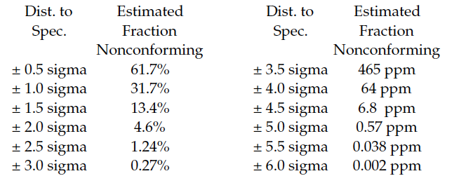
Figure 1: Traditional sigma levels

The first thing to note from Figure 1 is that the estimates are spread out over nine orders of magnitude. This will complicate the job of obtaining reliable estimates.

By using sigma levels to characterize the process fraction nonconforming, it would seem that Six Sigma programs are using the traditional approach. However, they add a completely spurious assumption.

The spurious 1.5 sigma shift

The sigma levels commonly quoted in Six Sigma training classes are shifted 1.5 sigma relative to those in Figure 1. For example, a “Six Sigma” process is said to be producing no more than 6.8 ppm nonconforming. This 1.5 sigma shift is said to allow for an unpredictable process. However, this claim is completely without foundation in either theory or practice. When a process is operated unpredictably, there is no magic-sized shift that can compensate for the unplanned process changes.

The example in last month’s column had subgroup averages that varied from 5 sigma(X) below the average to 10 sigma(X) above the average. Other examples from my clients show shifts of plus or minus 8 or 9 sigma, and one example has shifts of up to 30 sigma. Reality is not limited to shifts of 1.5 sigma or less. Never has been. Never will be.

So while this spurious 1.5 sigma shift is a problem with the sigma levels of Six Sigma, it is not the most serious problem. To understand the fundamental problem of sigma levels, we must look at how histograms and probability models work.

Your empirical distribution

A histogram summarizes the past performance of your process. The histogram is your empirical distribution. The data are your reality. Consequently, the best estimate of the fraction nonconforming is the binomial point estimate:

This binomial point estimate uses all of the information about the fraction nonconforming that’s contained in your data. As we noted last month, if you wish to extrapolate from your data to the product not measured, you’ll need to use an interval estimate (also known as a confidence interval). The preferred 95% interval estimate for a proportion is the Agresti-Coull interval estimate. This estimate is centered on the Wilson point estimate.

And the 95 Agresti-Coull interval estimate is computed as:

Unlike other interval estimates, the Agresti-Coull interval estimate works all the way down to Y = 0, which makes it useful here.

While the binomial point estimate is your best single value, the interval estimate defines the uncertainty in the point estimate associated with your extrapolation beyond the data.

This approach is completely empirical. Although it does implicitly assume your data to be homogeneous, it makes no assumptions regarding the shape of the distribution, and no assumption about a probability model for the data. The binomial point estimate and the Agresti-Coull interval estimate summarize the information contained in the data. They define what you know, and the limitations on that knowledge.

How probability models work

A probability model is a limiting characteristic for an infinite sequence of independent and identically distributed random variables. As the limit of an infinite sequence, a probability model can never be said to be a property of any finite portion of that sequence!

A unique, limiting probability model only emerges as the sequence becomes infinite. Any finite sequence will be consistent with several different probability models. The shorter the sequence, the greater the number of possible probability models.

Against this mathematical fact of life, we have to work with data that are always finite in number and extent. As a result, we can never fully specify a unique probability model as applying to our data. We simply will never have enough data to do so. This means that there is never just one right probability model. We will always have to make a choice when we fit a probability model to the histogram of our data.

The role of a probability model

When we choose a probability model to fit our histogram, we want a reasonable agreement across the bulk of the data. If the model doesn’t match the middle 90% to 99% of the data, it will not be of much use. But regardless of how well our model fits the bulk of the data, when it comes to the tails we have a problem. Histograms always have finite tails. Every histogram has a minimum and a maximum. Yet most continuous probability models have at least one infinite tail. Thus, there will usually be a discrepancy between the finite tails of our histogram and the infinite tails of our probability model. This discrepancy creates problems in practice. As the model goes beyond the last point in the tail of a histogram, it loses all contact with reality.

Out beyond the last point in our histogram, the shape of the tail of the model is entirely dependent upon which model we have chosen. Different models will have radically different tails. So, when we compute the infinitesimal areas in the extreme tails of our probability models, we are computing values that are based on our assumptions rather than being based on our data.

To illustrate this point, consider the 250 values in Figure 2. This histogram has an average of 7.4 and a standard deviation of 5.2. Clearly these data have a boundary condition on the left, resulting in a skewed histogram.

Figure 2: Histogram of 250 values

First, we consider fitting a lognormal distribution to these data. Since the median for the data is 6, we use a lognormal distribution with alpha = 6. To get an average of 7.4 we let beta = 0.65. This distribution has an average of 7.4 and a standard deviation of 5.37. The resulting fit is shown in Figure 3.

Figure 3: A lognormal model

A gamma distribution with alpha = 2 and beta = 2 (also known as a Chi-square distribution with four degrees of freedom) has a mean of 4 and a standard deviation of 2.828. When we stretch this distribution out 185%, we get a distribution with a mean of 7.4 and a standard deviation of 5.23, which results in the fitted model shown in Figure 4.

Figure 4: A gamma model

Finally, a Weibull distribution with alpha = 1.5 and beta = 8.2 will have an average of 7.4 and a standard deviation of 5.03. This model is shown in Figure 5.

Figure 5: A Weibull model

Figure 6 shows that these models differ the most on the left-hand side. They become quite similar in the middle and virtually indistinguishable in the upper tail.

Figure 6: Three models compared

The largest value in the data set is 27. So, areas under these curves to the right of 27.5 are areas from the region beyond the data.

If the upper specification limit is 28.5, then the traditional sigma level would be 4.05, P_pk would be 1.35, and the three models would yield estimates of the fraction nonconforming of 8,262 ppm, 3,808 ppm, and 1,947 ppm, respectively. Here the largest estimate is more than four times the size of the smallest estimate. So, which one should you use?

If the upper specification limit is 33.5, then the traditional sigma level would be 5.01, P_pk would be 1.67, and the three models would yield estimates of the fraction nonconforming of 4,075 ppm, 1,130 ppm, and 357 ppm, respectively. So, here the largest estimate is more than 11 times the size of the smallest estimate. (Of course, the six-sigma answer would be 465 ppm.) Which answer is right?

Finally, if the upper specification limit is 39.5, then the traditional sigma level would be 6.18, P_pk would be 2.06, and the three models would yield estimates of the fraction nonconforming of 1,870 ppm, 257 ppm, and 39 ppm, respectively. So, here the largest estimate is almost 48 times the size of the smallest estimate. The answer you get has no relationship to the data. It only depends upon your choice of a probability model. Estimates that vary by one or two orders of magnitude depending on an unverifiable assumption are not very reliable.

Once you go beyond the finite tails of your histogram, you have left the world of data analysis and entered the realm of mathematical make-believe. While you can always calculate infinitesimal areas in the extreme tails of your assumed probability model, you will have lost contact with reality along the way. The values you get will be an artifact of the model you’ve chosen rather than a property of the underlying process generating your data.

What your data will support

If we try to estimate proportions that correspond to values beyond the last point in our histogram, the point binomial estimate becomes zero, and the 95% A–C interval estimate formula for the upper bound on the fraction nonconforming becomes a function of how many data are being used:

For large n this is approximately:

When you estimate the fraction nonconforming, you’re making a prediction. And the upper bound above defines the inherent uncertainty in that prediction. Figure 7 lists these upper bounds on the estimated fraction nonconforming when the binomial point estimate is zero.

Figure 7: Ultimate 95% upper bounds on fractions nonconforming

So the estimates above, which ranged from 8,262 ppm to 39 ppm, can all be said to have an uncertainty of up to 19,000 ppm. That’s the precision these 250 data will support. When the uncertainty is two to 500 times the size of the estimate, that estimate is worthless.

With 5,000 or fewer data, when you go beyond the end of your histogram you can only support parts per hundred or parts per thousand estimates. To get estimates good to one part per ten-thousand (100 ppm), you would need at least 48,000 data in your histogram!

It is true that the probability of nonconforming product will become vanishingly small when a process is operated predictably and the capabilities increase beyond 1.10. However, you’ll never have enough information to begin to reliably quantify these vanishing probabilities until you can do so with a point binomial estimate that’s greater than zero.

So what about sigma levels

Figure 8 reproduces Figure 1. The traditional sigma levels in the left-hand column provide a reasonable way to characterize nonconforming product. However, the right-hand column does not. While the numbers in the right-hand column are computed correctly, they no longer represent reality. The uncertainty in the extrapolation from your data to your model simply overwhelms these infinitesimal values.

Figure 8: Traditional sigma levels

Probability models can provide useful estimates of a proportion in terms of parts per hundred or parts per thousand. But out beyond the ends of the histogram, they cannot be said to accurately represent any actual process. The infinitesimal areas in the extreme tails of an assumed probability model are simply complex estimates of zero.

So what should you do?

You should immediately stop using sigma levels to represent fractions nonconforming. The only sigma levels that approximate reality are the traditional sigma levels that come from a process that has demonstrated predictable operation, and which are less than 3.0. Estimates of the fraction nonconforming computed from a probability model that are less than one part per thousand are fictitious artifacts of the chosen probability model. They have no contact with reality. Do not believe or use them.

Instead of sigma levels, use performance indexes to describe the past process performance. Use capability indexes to describe the process potential. The gaps between the performance indexes and the capability indexes define the existing opportunities for process improvement.

Use process behavior charts to discover how to operate your process up to its full potential.

Use the point binomial estimate and the Agresti-Coull interval estimate to describe the past process nonconforming when your process is operated unpredictably. And, if you happen to already be operating your process predictably, you may also use these estimates of the process nonconforming as predictions of what to expect.

Donald J. Wheeler’s complete “Understanding SPC” seminar may be streamed for free; for details, see spcpress.com.