Social Sharing block
I
n my February 1996 Quality Digest column I discussed an article out of USA Today. Since that article provides a great example of how we need to filter out the noise whenever we attempt to interpret data, I have updated it for my column today. “Teen Use Turns Upward” read the headline for a graph appearing in USA Today on June 21, 1994. The data in the graph were attributed to the Institute for Social Research at the University of Michigan and were labeled as the “percentage of high-school seniors who smoke daily.”
The portion of this graph covering the 10 years from 1984 to 1993 is shown in figure 1.
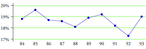
Figure 1: Percentage of high-school seniors who smoke daily
Each point in figure 1 is the value found in an annual survey. The 1993 value of 19.0 percent was higher than the 1992 value of 17.3 percent. This was interpreted to mean that more teenagers are using tobacco now than in the past. But are they?
…
Comments
Wood for my fire
Dear Donald,
Thanks for reminding me of this article. It certainly gives me wood for my fire. (it will be forwarded to some people that should read it) I do a lot of work in marketing and sales. It is possibly the industry where understanding variation should be crucial. I have witnessed Companies "losing" millions by either not even measuring or acting on single events without understanding the context.
I would be interested in your own and your readers experience in applying XmR charts on sales and marketing data.
Kind Regards
Francois van der Walt
2.66 and 3.27
Hello Dr. Wheeler:
Do the constant values of 2.66 and 3.27 have names? I would like to better understand where these constant values come from.
Thank you, Dirk van Putten
Great Article
Hello Dr. Wheeler:
Great article by the way. I followed all of the math and statistics and understood the genreal concept of noise vs. signal.
Thank you, Dirk
Scaling Factors
Hello Dr. Wheeler:
I think I found my answer in your Book, "Twenty Things You Need To Know", Chapter 5, Where Do Scaling Factors Come From?
Thank you, Dirk
Constant Values 2.66 and 3.27
Dirk Van Putten, 2.66 is 3 / d_2, where d_2 is an anti-biasing constant that can be found in most textbooks. 3.27 is the D_4 anti-biasing constant.
The Wikipedia page on Indivduals charts (https://en.wikipedia.org/wiki/Individuals_chart) gives a decent overview the charts. Dr. Wheeler's books and other writings go into somewhat greater detail on the constants, as do other books on statistical process control (see, for example, the classic text by Montgomery, though I would caution that Montgomery's general approach to process behavior charts sometimes seems to be at odds with Dr. Wheeler's).
XmR charts on sales and marketing data
Hi Francois van der Walt,
I have used XmR charts on sales and marketing data, and I could email examples to you if you want (Spanish). You may also visit Pauls Selden's web page: www.paulselden.com He is author of several works in the field, including "Sales Process Engineering".
For Francois van der Walt
2.66
Detecting change in successive surveys
The article shows the use of I-MR charts to detect change. With survey data, what is the role of confidence intervals when deciding if there has been a change between successive survey averages?
To use the teens smoking example, what if we had a 99% confidence interval of +/-0.5% for each year of survey data. Then we move from 17.3% in '92 to 19.0% in '93. Should we be able to say we're 99% confident that the 1992 and 1993 smoking rates are different? Or, in this case, as the I-MR chart shows we cannot conclude there is a change, is our only our conclusion that the difference from 1992 to 1993 is not due to survey error, it's just common cause variation in the underllying process.
Should be required reading
This article should be required reading for every journalist, journalism major and blogger. Also every government employee, politician, lobbyist and spind doctor. Actually, some of those folks probably understand these things and try to use it to advantage (that would be the "damned lies" part).
Add new comment