In order to do business, we have to use predictions of various sorts. These range from seat-of-the-pants guesses to the results of sophisticated modeling. In every case, the key to effective forecasting is to understand the uncertainty in the forecast. Ways to do this are the subject of this article.

For many years I taught the senior-level forecasting course in the college of business at the University of Tennessee. In that class, we covered many different techniques for massaging the data to obtain forecasts. Regardless of the complexity of the technique used, the limiting factor in every forecast was always the noise in the data themselves. The various techniques would provide exact values, but these values would only be as good as the uncertainty in the source material.

There are basically two approaches to forecasting. One simply uses the data themselves to make a forecast. We will call this an empirical approach. The other approach creates some model for the data and uses the model to make a forecast. Both approaches are valid, and both have their place. But neither gives forecasts that are more precise than the variation present in the data will allow. This means that getting the forecast is only half the job. The forecast is incomplete until you also know how much uncertainty to attach to the forecast.

Aggregated data

Managers usually deal with highly aggregated values. Highly aggregated time series tend to be fairly predictable, but they also tend to contain so much noise that the predictions are not very precise. For an example, consider the quarterly sales figures for one company (in thousands) shown in Figure 1.

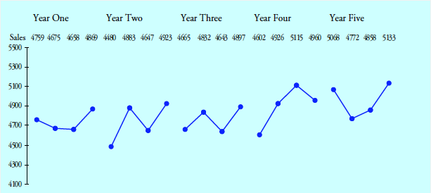
Figure 1: Quarterly sales

What would you forecast for the first quarter of Year 6? Intuitively, we turn to averages. We might use the average over the past five years of 4,818. Or we might use the average over the last year of 4,958. While the actual value is unlikely to fall right at either of these averages, they give us a ballpark forecast.

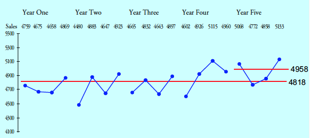
Figure 2: Two empirical forecasts for Y6 QI

Once you notice that six of the first 10 quarters are below the five-year average, while seven of the last 10 are above this average, you might wish to create a trend line to use in forecasting. The recommended way to do this is to compute the average for the first half of the data (4,739) and plot this point at the midpoint of the first-half time periods (time period 5.5). Next, compute the average for the second half of the data (4,897) and plot this at the midpoint of the last-half time periods (time period 15.5). Connecting these two points gives your trend line model. The difference between the averages divided by the number of time periods between them gives a trend per time period of 15.9 units per quarter. Extending this out to the first quarter of Year 6 produces a model-based forecast of 4,984.

Forecast Y6 QI = 4,897 + 5.5 (15.9) = 4,984

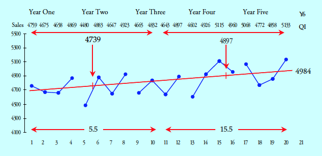
Figure 3: A model-based forecast for Y6 QI

Now we have three forecast values. How do we choose between them? Before we try to do this, it helps to understand how much uncertainty is attached to each.

Characterizing uncertainty

The preferred way to characterize the variation in a time series is the method of  successive differences (also known as moving ranges). A moving range is the absolute value of the difference between successive values. Once we have computed the moving ranges, we use the average moving range to compute the number of measurement units in a standard unit of dispersion. This quantity is commonly known as sigma (or the standard deviation). For the sales data, the average moving range is 222 units, and sigma is:

This value tells us that a standard unit of dispersion for our time series contains 197 measurement units. This value is the key to effective forecasting.

While there are many different ways of computing estimates of a standard deviation, they are not all equivalent in practice. To avoid getting inflated estimates of dispersion, you should always use the method of successive differences when working with time series.

Stationary time series

A stationary time series is one where the past will provide a reliable guide to the future. For a stationary time series, the empirical rule tells us to expect two-thirds or more of the values to fall within one sigma unit of the central line. (See appendix below for empirical rule.) We can use this to compute an interval forecast for the most likely values.

For the sales data, based on our trend line forecast, our most-likely forecast for QI of Year 6 is the interval:

Most-likely forecast interval = 4,984 ± 197 = 4,787 to 5,181

Since this interval contains the two empirical forecasts, we have to conclude that we cannot distinguish between our three earlier forecast values.

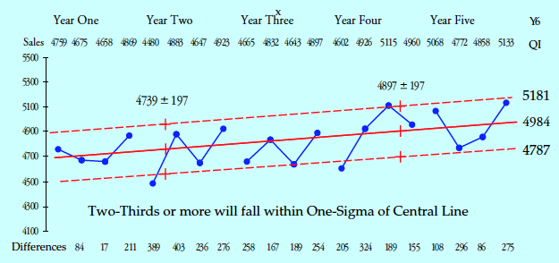
Figure 4: A most-likely forecast for Y6 QI

“Can’t we predict any more precisely than that? Plus or minus 200 is not very useful.”

Look at Figure 4. How well do the two dashed lines describe the past? While three points are outside these one-sigma lines, four more are very close, leaving 65% comfortably within the lines shown. Plus or minus 197 units is the inherent uncertainty in this time series, and we have to allow for this when we forecast the future.

If you want better odds than two out of three, you’ll need a wider interval. For a stationary time series, the empirical rule tells us that the observations will fall within two sigma units of the central line about 95% of the time. So a 95% forecast interval will be the central line forecast plus or minus two sigma units.

95% forecast interval = 4,984 ± 394 = 4,590 to 5,378

The least favorable end of the 95% forecast interval is especially useful when management wants to be able to report that they have “exceeded the forecast.” However, don’t be fooled by this game. The best single value for internal use is still the central line.

Finally, for a stationary time series, the empirical rule tells us that approximately 99% to 100% of the observations will fall within three sigma units of the central line. In this way, we can compute worst case/best case limits:

Worst/Best forecast = 4,984 ± 590 = 4,394 to 5,574

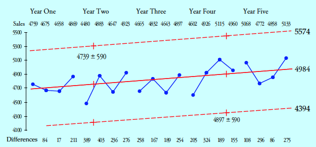
Figure 5: Worst/Best forecast for Y6 QI

Usually these worst/best limits are far too wide to be of much use as a forecast. But they will serve to help you identify when your time series is no longer stationary. When a point goes outside the worst/best limits, you have strong evidence that the underlying processes creating the time series have changed. Such changes mean that your model-based and empirical forecasts may no longer be appropriate.

Reducing uncertainty

Highly aggregated time series tend to be stationary simply because they tend to be full of noise. This noise makes the forecasts so broad that they are hardly useful. So how can we do better? One thing that can be done is to disaggregate the time series and look at the various components separately.

The company of Figure 1 had six sales offices. We shall look at the sales for three of these offices, beginning with Region D.

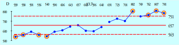
Figure 6: XmR chart for quarterly sales for Region D

The five-year average for Region D is 657. The average moving range is 35, so sigma is 31.2 units. The eight points outside the three-sigma limits in Figure 6 suggest an upward trend for these data. When we compute a trend line and attach the worst/best limits, we find a stationary time series with an upward trend of 13.7 units per quarter.

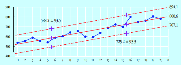
Figure 7: Quarterly sales trend for Region D with worst/best limits

With this model, a point forecast for the first quarter of Year 6 for Region D is:

Forecast for Y6 QI = 725.2 + 5.5 (13.7) = 800.6

And the most likely interval is:

Most likely forecast interval = 800.6 ± 31.2 = 769 to 832

Region C

The first four years for Region C show an average of 1,191 and a sigma of 88. With seven of the first eight points below the average, and the next-to-last point above the best case limit, we have evidence of an upward trend.

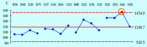
Figure 8: XmR charts for Region C sales for years 1–4

These four years yield a trend line that is increasing 20 units per quarter. But when we plot the values from Year 5 on this graph, we find evidence that the trend is no longer appropriate.

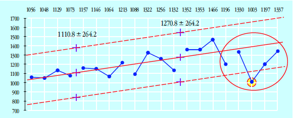
Figure 9: Region C sales trend with worst/best limits

The departure from the trend is detected in the second quarter of Year 5. It could have started as early as the fourth quarter of Year 4. So, for purposes of forecasting, we abandon the trend line and return to using the average of 1,212 from the last five quarters as our central-line forecast.

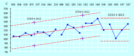
Figure 10: Region C worst/best limits for Year 6

Here, the most-likely forecast for the first quarter of Year 6 for Region C would be 1,124 to 1,300 units.

Region A

Region A sales would be stationary except for a pattern that recurs every two years. This pattern should be incorporated into any forecast.

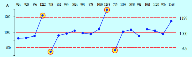
Figure 11: XmR chart for Region A sales

The average is 1,000, and sigma is 65, which gives the worst/best limits shown. But every two years, they end with a big fourth quarter followed by a disastrous first quarter. Since the last quarter of Year 5 is up near the best case limit, I would forecast the next quarter to be near the worst case limit of 805, with a most likely interval forecast of 740 to 870 units.

Recurring patterns are commonly known as seasonal effects. Next month’s column will discuss ways to use seasonal effects in forecasting.

Summary

Report-card time series tend to be highly aggregated. This makes them both relatively predictable and full of noise. When working with time series over which we have little to no control, we can still use the data to make reasonable forecasts. However, until we understand the inherent uncertainty in these forecasts, we will be prone to overinterpret their precision.

All data are historical. All analysis of data describes the past. Prediction requires extrapolation from the past to the future. A stationary time series is one where the past provides a reliable guide to the future.

Three sigma limits provide a test to see whether a time series continues to be stationary. When points exceed the worst case/best case limits, something has changed, and the old forecasting model may no longer work.

However, even with a nonstationary time series, patterns within the data may be used to find reasonable forecasts. The graph reveals things that no amount of computation will ever detect. So the first step in forecasting is to start with your data on an XmR chart and see what your data can tell you.

Appendix: The empirical rule

For those who may not be familiar with the empirical rule, the following may be helpful. Certain minimum percentages can be established for central intervals of unimodal probability models that are suitable for use with original data. The following figures summarize the results of looking at over 5,000 such probability models. The 20 models shown are representative of the shapes considered in the study. The horizontal scale shows the distance to the mean in sigma units.

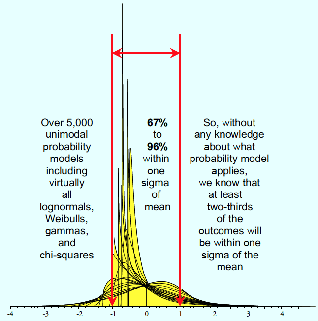
Figure 12: Part 1 of the empirical rule

A normal distribution has 68.3% within one sigma of the mean. This is near the minimum for distributions with at least one infinite tail. Consequently, the normal distribution has a maximal amount more than one sigma away from the mean. This is part of what it means when we say the normal distribution is the distribution of maximum entropy. While the central limit theorem tells us that the normal is the limiting distribution for many phenomena, the fundamental nature of the normal distribution is revealed when we understand that the central limit theorem is simply a restatement of the second law of thermodynamics.

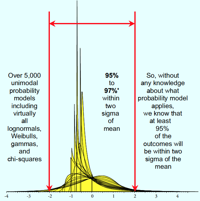
Figure 13: Part 2 of the empirical rule

Unimodal distributions that are suitable for describing the original data will have at least 95% within two sigma of the mean. Most of these distributions have between 95% and 96%, making the normal distribution value of 95.45% a nearly universal average.

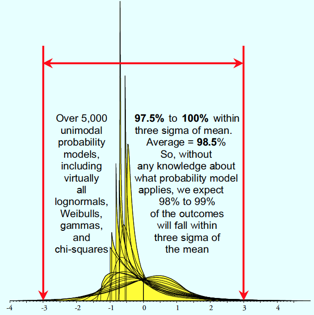
Figure 14: Part 3 of the empirical rule

Once again, most of the models had more than 98.5% within three sigma. So, without having to know what probability model to use, you can safely say that at least two-thirds, approximately 95%, and approximately 99% will be found within one-, two-, and three-sigma of the mean.

These percentages work because the standard deviation is the radius of gyration for a distribution, and you cannot cheat on rotational inertia: Certain minimum percentages have to fall in intervals of various widths centered on the mean.

Donald Wheeler’s complete “Understanding SPC” seminar may be streamed for free. For details see spcpress.com.