When a time series displays a pattern that repeats itself periodically it is said to have seasonal effects. The word seasonal may apply to days, weeks, months, quarters, or any pattern that recurs regularly throughout the data. While these seasonal effects will complicate our analysis, their regularity can be utilized to improve our forecasts. Two ways of doing this are the topic of this article.

Smoothing seasonal effects

A simple way to deal with seasonal effects is to average them out. If your data show a recurring pattern every p time periods, use a p-period moving average to reveal the underlying trend over time. Figure 1 contains a set of quarterly data along with the four-period moving averages for those data.

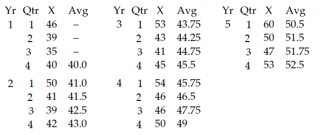
Figure 1: Five years of quarterly data

These data show a seasonal pattern while the four-period moving averages show an upward trend.

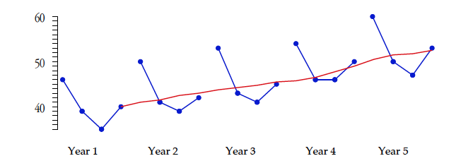
Figure 2: Quarterly data and moving averages

Computing the average difference between successive moving averages, we find that this trend is increasing 0.78 units per quarter. Adding this amount to the last moving average creates an estimate for the first quarter moving average for Year 6 of 53.28. This, in turn corresponds to a forecast first quarter value of 63.1.

If we are willing to assume that the trend will continue as before, we can extend our extrapolation into the future one quarter at a time. However since each step would be built on the one before, these forecasts will be increasingly uncertain.

Assuming the moving averages increase 0.78 units per quarter during Year 6, we estimate moving averages to be 53.28, 54.06, 54.84, and 55.62. Based on the observed values in Year 5, these estimated averages result in forecast values of 63.1, 53.1, 50.1, and 56.1 for Year 6. This approach to forecasting uses the moving average as a floating trend line plus the seasonality of the sales over the most recent year. With these rather minimal assumptions, you can get reasonable forecasts that will generally be as accurate as those coming from more complex model-based approaches.

Estimating seasonal effects directly

Moving averages provide a quick and straightforward way to smooth out seasonal effects. The alternative is to directly estimate each of the seasonal effects and use these effects to deseasonalize the time series. This model-based approach is the one commonly taught in business schools.

To estimate seasonal effects, you’ll need at least two, and usually not more than five, years’ worth of data. The years used to estimate the seasonal effects will be known as the “baseline years.” Here, we’ll use the first three years of Figure 1 as our baseline.

We begin by computing the seasonal relative for each quarter for years 1, 2, and 3 in Figure 3. The seasonal relative is the quarterly value divided by the average quarterly value for that year.

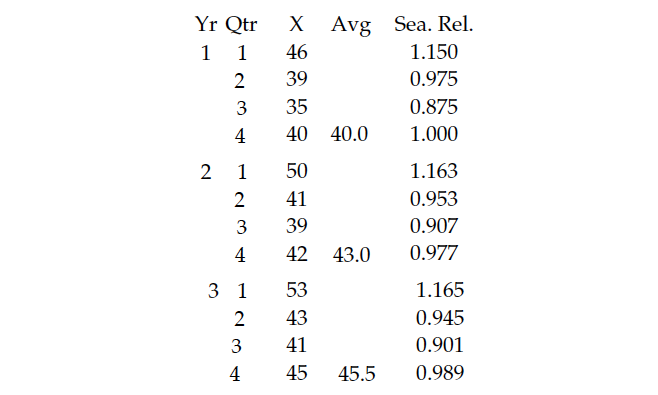
Figure 3: Seasonal relatives

There’s no point in computing seasonal relatives to more than three decimal places, since we’re going to average and adjust them before use. The next step is to determine whether the seasonal effects are real or just random variation. This is done by placing them on a special average and range chart. This chart will have one subgroup for each season. The subgroup size will be equal to the number of years in the baseline period, denoted here by m. So our average and range chart has four subgroups of size 3, and is shown in Figure 4.

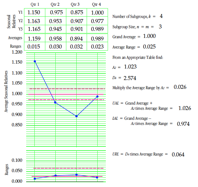
Figure 4: Average and range chart for seasonal relatives

This average and range chart is not a traditional process behavior chart. Instead, it’s a chart organized to show the seasonal effects. The averages show the seasonal pattern in these data while the limits define the uncertainty in this pattern. Averages outside the limits represent detectable seasonal effects (Quarters 1 and 2). Averages on or near the limits may be interpreted as weak seasonal effects (Quarter 2). Averages comfortably within the limits represent seasons with no detectable seasonal effect (Quarter 4).

The limits of ±2.6% on the average chart suggest that these data are sufficient to detect seasonal effects that deviate from the grand average by more than ±2.6%. With uncertainties of 2% or so in our estimates, we round them off to two decimal places for use. Thus, we have detectable seasonal effects of 1.16, 0.96, and 0.89 for the first three quarters.

To avoid inflation or deflation in our forecasts the sum of the seasonal effects must always equal the number of seasons. Since our three detectable effects add up to 3.01, we’re left with 0.99 to use as our seasonal effect for the fourth quarter. So while we don’t have a detectable seasonal effect for the fourth quarter, we still round it off to 0.99 to have a balanced set of seasonals.

Once we have estimated seasonal effects, we may deseasonalize the data by dividing each value of the baseline years by its appropriate seasonal. This allows us to see any underlying trends within the baseline period more clearly.

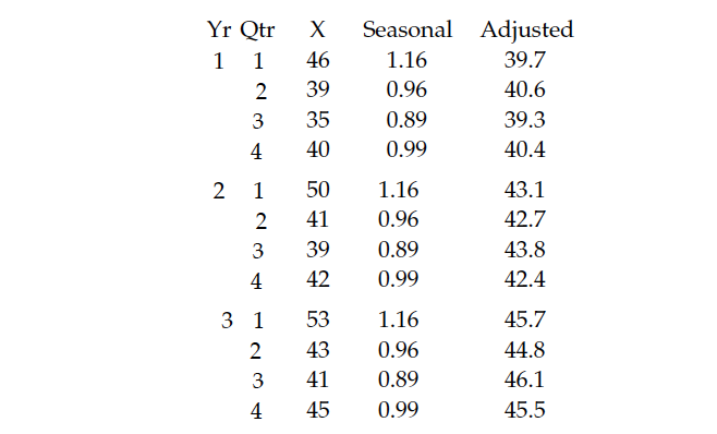
Figure 5: Deseasonalized years 1 to 3

Plotting the average of 40 for Year 1 at the midpoint of Year 1, and plotting the average of 45.5 for Year 3 at the midpoint of Year 3, we find the trend line shown in Figure 6. This trend line is increasing 0.69 units per quarter.

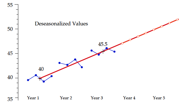
Figure 6: Deseasonalized years 1 to 3

The trend line provides estimates of the deseasonalized future values as shown by the white dots in Figure 6. These trend line values can be multiplied by the seasonal effects to obtain forecast values for each quarter of years 4 and 5.

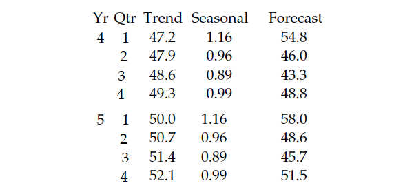
Figure 7: Forecast values for years 4 and 5

Figure 8 shows these forecast values (red) as well as the actual data (blue) from Figure 1.

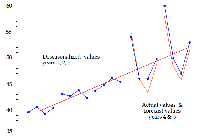
Figure 8: Forecast vs. actual for years 4 and 5

This model-based approach to forecasting synthesizes reasonable forecasts based on the past time-series values. Because it’s built on multiple assumptions, the uncertainty of these forecasts will generally exceed any estimate thereof coming from the mathematical background. So, rather than trying to synthesize a measure of uncertainty for these forecasts, it will generally be best to empirically measure them. The average of the absolute values of the differences between actual results and forecast results for years 4 and 5 is 1.36 units. With this amount of observed uncertainty, we might expect most forecasts to be within twice this distance of the actual values.

Charting deseasonalized values

The time to revise our model of a time series is when a change has occurred—and the best way to determine if a change has occurred is to use a process behavior chart with the deseasonalized data. To place the baseline years deseasonalized values on an XmR chart, we have to compute the moving ranges as shown in Figure 9.

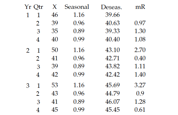
Figure 9: Deseasonalized years, 1 to 3, and moving ranges

The average moving range is 1.36. Multiplying by 2.66 results in three-sigma limits 3.62 units on either side of the trend line in Figure 10.

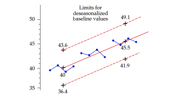
Figure 10: Limits for deseasonalized baseline years

To see whether a change has occurred following this baseline period, we deseasonalize the subsequent future values as they occur, and then place them on an extension of the chart in Figure 10. Figure 11 shows the actual values from years 4 and 5 along with their deseasonalized values.

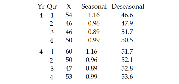
Figure 11: Deseasonalized values for years 4 and 5

While the limits shown in Figure 10 are the correct limits for the baseline deseasonalized values, they’re not the correct limits to use with the deseasonalized future values of Figure 11. The limits in Figure 10 are deflated by the correlation created when we adjusted the baseline years using the seasonals obtained from the baseline years. To use the average moving range from the baseline years to compute limits for future values, we have to undo this deflation. The amount of deflation depends upon the number of years in the baseline period, denoted here by m. The central line for the X chart remains unchanged. The X chart limits for future deseasonalized values computed from the baseline average moving range will be:

And using the average moving range from the baseline deseasonalized values, we find the limit and central line for the successive differences of future deseasonalized values to be:

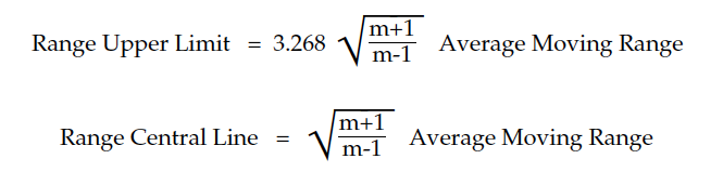
For our example m = 3, and our average moving range was 1.36, so our limits on the X chart will be ± 5.12 either side of the trend line. These limits are shown in Figure 12.

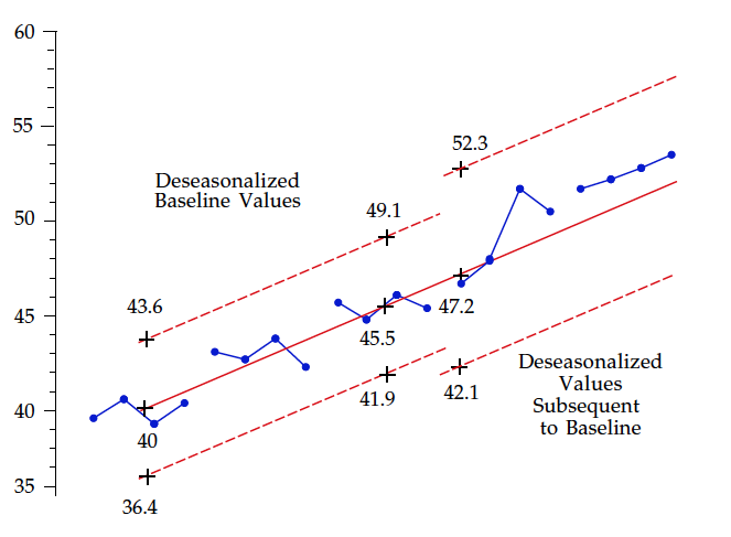
Figure 12: Limits for deseasonalized future years

While we have six quarters in a row above the trend line, we still don’t have enough evidence to be sure that we need to revise the trend line or seasonal effects here. However, decisions about updating a model are always subjective. Here, we might decide to adjust the trend line up by 1.5 units to better accommodate the most recent data. If we did that and extended this trend line into Year 6, we would end up with forecasts of 62.7, 52.8, 49.7, and 55.8.

Caveat

The moving average approach came up with forecasts of 63, 53, 50, and 56 for Year 6. The only practical difference between these forecasts and those in the previous paragraph produced by the traditional model-based approach is the effort required to obtain them.

The quality of a forecast is generally determined by the noise within the data rather than the complexity of the forecasting technique. So don’t get carried away by complex models for forecasting. The following is an example of what can happen if you do.

Perry got some new software that allowed him to fit an auto-regressive integrated moving average (ARIMA) to his data. He decided to use it to forecast the residual viscosity of a distillation column. After playing with the software for two weeks, Perry finally obtained a satisfactory ARIMA model. Using his model, he could obtain a 95% interval estimate for the next value as:

When Perry brought his model to me, I used his data to create the XmR chart in Figure 13. With limits based on the first 10 values, we see a process that has gone on walkabout.

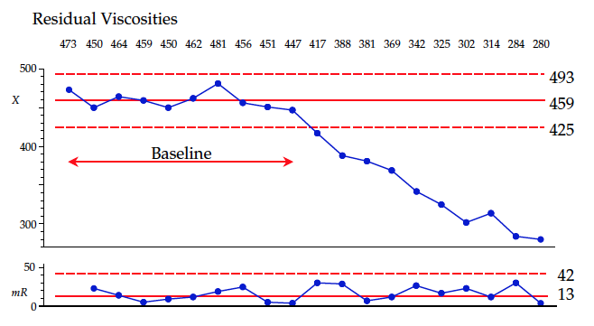
Figure 13: XmR chart for residual viscosities

In spite of these changes, the moving ranges all remain below the upper range limit. Data like these tend to have a vary large lag-one autocorrelation. Here, we can use the current value of the time series as our point forecast for the next period, and use the upper range limit as our 99% uncertainty on that forecast, resulting in a prediction of:

Why did the ARIMA model have nearly twice the uncertainty?

When we fit a model to our data, there will inevitably be some “lack of fit” between the model and the data. This lack of fit will always increase the uncertainty in our forecasts. It can do no other. While the ARIMA model is sophisticated and impressive, it introduced more noise than it explained. Any model is useful only to the extent that it explains more variation than it introduces into the forecasts.

Summary

Simple moving averages allow you to smooth out seasonal effects. The traditional approach of directly estimating the seasonals will allow you to work with seasonal effects effectively. Greater complexity is seldom needed.

The purpose of analysis is insight, and the best analysis is always the simplest analysis that gives the needed insights.

See Part 1: The Art of Forecasting

Donald Wheeler’s complete “Understanding SPC” seminar may be streamed for free. For details see spcpress.com.