That’s fake news. Real news COSTS. Please turn off your ad blocker for our web site.
Our PROMISE: Our ads will never cover up content.
Donald J. Wheeler
Published: Monday, December 2, 2013 - 17:05 It would appear that there is still considerable confusion regarding which method to use in evaluating a measurement process. There are many voices speaking on this subject, however, most of them fail to use the guidance provided by statistical theory, and as a result, they end up in a train wreck of confusion and uncertainty. Here the three most common methods will be compared side by side. Our example will use the data obtained from a gauge used to measure gasket thicknesses in mils. Three operators measure five parts two times each to obtain 30 measurements arranged into 15 subgroups of size 2 as shown in figure 1. To understand these data it is helpful to observe that the operator-to-operator differences show up between the subgroups, the part-to-part differences show up between the subgroups, and the test-retest error shows up within the subgroups. This organization is the key to interpreting these data. The comparison between the three approaches to gauge repeatability and reproducibility (R&R) studies will be carried out in two phases. In the first phase we shall look at the estimates of the various components of variation, and in the second we shall look at how the three approaches use these estimates to characterize the relative utility of the measurement system for a given application. The analysis of variance (ANOVA) approach to gauge R&R uses software to carry out the complex computations. This makes it a black-box technique. Once you have figured out how to enter the data above into the software correctly, the program will spit out an ANOVA table like that in figure 2. The large F-value for parts (having a P-value less than 0.05) tells us that the measurement system can detect the differences between the five parts used in the study. This is good news because we want to be able to detect the part-to-part differences over and above measurement error. The large F-value for operators tells us that there is a detectable operator effect present and the three operators are not measuring the parts the same. Specifically, the three operators do not all agree on the average value for the set of five parts. This is bad news. An operator effect is a nuisance component of measurement error. Although the ANOVA approach detects this operator effect, it does not tell you which operator is out of line with the others. The nonsignificant F-test for interactions is another bit of good news. You do not want the operators to interact with the parts. If the operators measure the same parts differently you have a serious problem with your measurement process that will need to be fixed before the measurement system will be of any real utility. ANOVA repeatability: Our ANOVA estimate of the repeatability standard deviation or test-retest error has 15 degrees of freedom and is simply the square root of the mean square within (MSW): ANOVA reproducibility: Since we have a detectable operator effect our ANOVA estimate of the reproducibility standard deviation has two degrees of freedom and is found by using the mean square for operators (MSO), the mean square for interactions (MSI), and the mean square within (MSW): ANOVA product variation: If we think that the five parts used in this study are reasonably representative of the product stream we might use them to estimate the standard deviation of the product stream. This estimate would have four degrees of freedom and would be found using the mean square for parts (MSP), the mean square for interactions (MSI), and the mean square within (MSW): ANOVA total variation: The three components of variation above may be combined to create an estimate of the standard deviation of the product measurements: Because the computations for ANOVA can be extremely sensitive to round-off error, different software packages can give different results. I recently read a dissertation produced earlier this year that had to compare the ANOVA results from different software packages because they gave different results. When black-box approaches disagree, it is always hard to determine which result is correct if you cannot perform the computations required. The Automotive Industry Action Group (AIAG) has been in the business of interpreting statistics for industry since 1990. Their approach to the data of figure 1 consists primarily of computations of the estimates above and the computation of interpretative quantities. Their first step is to compute the upper range limit to check to see if any ranges from figure 1 exceed this upper limit. Here the average range is 4.267, the upper range limit is 13.9, and all of the ranges are less than this value. AIAG repeatability: Step 2 is to compute an estimate of repeatability using the average range. Here they divide by the traditional bias correction factor of d2 = 1.128 to get an estimate with 13.4 degrees of freedom of: AIAG reproducibility: Step 3 uses the operator averages to compute an operator range and then uses this to estimate the reproducibility standard deviation. The three operator averages are 181.0 mils, 172.5 mils, and 173.9 mils, respectively. The range of these three values is Ro = 8.5 mils. The bias correction factor used by the AIAG manual here is the bias correction factor for estimating variances which is commonly known as d2*. For the range of three values this value is 1.906. The reproducibility estimate will have two degrees of freedom and is: It should be noted that the AIAG approach computes the above number regardless of whether or not there is a detectable operator bias present in the data. While this value is appropriate in this case, this computation is inappropriate in the absence of a detectable operator bias. AIAG step 4 combines the repeatability and reproducibility: AIAG product variation: Step 5 uses the averages for each part to compute a part-to-part range and then uses this range to estimate the standard deviation of the product stream. The five part averages are 158.0, 206.167, 182.0, 184.833, and 148.0, respectively. The range of these three values is Rp = 58.167 mils. The bias correction factor used by the AIAG manual here is the bias correction factor for estimating variances, which is commonly known as d2*. This is done in spite of the fact that they are estimating a standard deviation. For the range of five values this value is 2.477. The product standard deviation estimate will have four degrees of freedom and is: AIAG total variation: Step 6 provides an estimate of the standard deviation of product measurements by combining the repeatability, the reproducibility, and the product variation: These estimates are compared with the estimates from other approaches in figure 6 below. Unlike the two preceding approaches, the “evaluating the measurement process” (EMP) approach begins with the average and range chart for the data of figure 1. This allows you to quickly see the interesting aspects of your data before you get overwhelmed by computed values. Figure 3: Evaluating the measurement process (EMP) chart for figure 1 In interpreting this chart it is important to understand that here we are using the average and range chart with experimental data. This means that we expect to see points outside the limits on the average chart—the whole point of doing an experiment is to create signals. At the same time, we do not want to see any signals on the range chart. Figure 4 shows what we look for on the EMP chart. This interpretation is due to the structure of these data. The operator-to-operator differences show up between subgroups. The part-to-part differences also show up between subgroups. The only source of variation left inside these subgroups is test-retest error, also known as repeatability. Thus, the limits on the average chart reflect that amount of variation which is obscured by measurement error. At the same time, the running record on the average chart shows the variation due to the product samples and the variation due to any operator differences that are present. Since we want to detect the product variation in spite of measurement error, we want to find points outside the limits on the average chart. The more points that are out, and the further out they are, the better we like it. Because the range chart checks for consistency within the subgroups, any signals on the range chart would indicate that the measurement process was inconsistent. This check for consistency is missing from the ANOVA approach—it simply assumes that the measurement process is consistent. At least step 1 of the AIAG method does check to see if there are any exceptional ranges. However, only the EMP approach actually constructs the range chart to show the consistency or inconsistency of the measurement process. In addition to having points outside the limits on the average chart, and having the ranges all inside the limits, we also look for reasonable parallelism between the operators. We want them to agree on which parts are high and which parts are low. We also would like the operators to all have similar averages. In figure 3 we have reasonable parallelism, but operator A is a little bit high compared to the other two operators. The reasonable parallelism in figure 3 corresponds to the nonsignificant F-value for the interaction effect in the ANOVA table. The higher average for operator A in figure 3 is the operator effect found in the ANOVA table in figure 2. How can we check to see if the operators all have the same average value for the five parts with EMP? We do this with an analysis of main effects (ANOME) chart. The analysis of main effects is an analysis of means (ANOM) technique explained in my February 2011 column “A Better Way to Do R&R Studies.” The grand average is 175.8 and the average range is 4.267. We have k = 15 subgroups of size n = 2. The m = 3 operator averages are 181.0, 172.5, and 173.9. With an alpha-level of 5 percent the ANOME scaling factor is 0.592, giving limits of: And clearly operator A is different from operators B and C. Since this difference in operators represents a nuisance component of measurement error, we will want to estimate the effect this has upon the quality of the measurements. Thus, we will need to estimate the reproducibility as well as the repeatability in this case. EMP repeatability: In an EMP study several different choices for computational formulas are offered. The following are what I typically use. An unbiased estimate of the standard deviation of measurement error having 13.4 degrees of freedom is: EMP reproducibility: For estimating the reproducibility I use the same approach as step 3 of the AIAG approach. Using the range of the three operator averages we end up with an estimate having two degrees of freedom: EMP product variation: For estimating the product standard deviation we use a formula that is slightly more precise than the one used in the AIAG study. The range of the five part averages is still 58.167, and the bias correction factor is still 2.477, but now we remove some bias that was ignored earlier. So, using the range of the part averages we obtain an estimate having four degrees of freedom: EMP total variation: As before, we combine the three estimates above to obtain an estimate of the standard deviation of the product measurements, which is: The table in figure 6 compares the estimates of these various quantities obtained from the three approaches. There is no practical difference between the various estimates of these four fundamental components of variation. The difference between the three approaches does not lie in the values found in figure 6, but rather lies in how these estimates are used to describe the relative utility of the measurement system. The quantities in figure 6 are estimates of the square roots of the variance components. In the ANOVA approach we square the estimates from the ANOVA column of figure 6 and express the first three numbers as a percentage of the last of these squared values to obtain a table of variance components as shown in figure 7. Since the last component is the sum of the first three components, it is customary to express each of the first three components as a percentage of the last component. ANOVA relative utility: Once we have the estimates found above we will want to use them to obtain a statistic that will characterize the relative utility of the measurement system for measuring this product. The standard statistic for this purpose is the estimate of the intraclass correlation coefficient. This statistic is found in figure 7: This value is properly interpreted to mean that the variation in the product stream accounts for 94.75 percent of the variation in the product measurements. Conversely, the repeatability and reproducibility combine to account for 5.25 percent of the variation in the product measurements. The intraclass correlation coefficient defines that percentage of the variation in the product measurements that is directly attributable to variation in the product stream. This fact makes it easy to explain in practice. The fact that it has a fine ancestry of high-brow mathematical statistics dating back to the 1920s makes it the traditional measure of relative utility of a measurement system for a given application. Accept no substitutes. With the EMP approach we end up with essentially the same estimates of the standard deviations for repeatability, reproducibility, and product variation as obtained from the other two approaches. As with the ANOVA approach we can square the values in the EMP column of figure 6 to create the table of variance components for the EMP approach seen in figure 8. Once again, we express each of the first three values as a percentage of the last value. Here our estimate of the intraclass correlation coefficient is 94.37 percent. So we estimate that about 94 percent of the variation in the product measurements is attributable to the variation in the product stream, and less than 6 percent is due to repeatability and reproducibility. Thus, the EMP approach yields an estimate of the intraclass correlation coefficient that is essentially identical to the value found using the ANOVA approach. Even though the numbers are slightly different, the overall interpretation remains the same with EMP as with the ANOVA approach. Thus, for measuring this product, this measurement system is already very good, and the impact of the operator difference is minimal. (If we are able to get operator A to operate in line with operators B and C, then the reproducibility component would go to zero, and the intraclass correlation coefficient would increase from 94.4% to around 97.5%.) The AIAG approach does not concern itself with the components of variance. Instead, It computes its own measures of relative utility by using the quantities from figure 6 directly. The AIAG approach computes ratios by dividing each of the first three AIAG values in figure 6 by the last AIAG value, 24.17. These values are then multiplied by 100 to obtain the AIAG “percentages” shown in figure 9. Then the repeatability and reproducibility percentages are compared to guidelines to determine the relative usefulness of the measurement system. The AIAG manual interprets the values in figure 9 to mean that repeatability consumes 16 percent of the total variation, reproducibility consumes 18 percent of the total variation, and the product stream consumes 97 percent of the total variation. Of course, the immediate problem with the three “percentages” in figure 9 is that they add up to 130 percent! Not knowing what else to do about this problem, the AIAG manual simply inserts a statement at this point to the effect that “The sum of the percent consumed by each factor will not equal 100%.” This statement has no explanation attached. There is no guidance offered on how to proceed now that common sense and every rule in arithmetic have been violated. Just a statement that these numbers do not mean what they were just interpreted to mean, and the user is left to his or her own devices. Unfortunately, unlike the Red Queen, when it comes to arithmetic we do not get to say that things mean whatever we want them to mean. To make sense of the AIAG “percentages” we have to construct a couple of right triangles as shown in figure 10. There the various estimates obtained by the AIAG approach are shown as the sides of the triangles. Figure 10: The quantities used by AIAG to compute pseudo-percentages Those who are familiar with high-school trigonometry will immediately recognize that the ratio of repeatability (3.783) to total variation (24.171) is the sine of angle A times the cosine of angle B. Likewise the ratio of reproducibility (4.296) to total variation is seen to be the sine of angle A times the sine of angle B. The ratio of product variation (23.483) to total variation is the cosine of angle A. So, in interpreting these ratios as percentages the AIAG group is effectively ignoring the Pythagorean theorem and confusing trigonometric functions with proportions. The fact that these numbers are irredeemable nonsense may be seen by comparing them with the true proportions given in figure 11. The repeatability consumes about 2.2 percent of the total variation rather than the 16 percent erroneously suggested by figure 9. The reproducibility consumes about 3.0 percent of the total variation, rather than the 18 percent erroneously suggested by figure 9. So what can you learn from the AIAG gauge R&R study? Virtually nothing that is true, correct, or useful. You have taken the time and gone to the trouble to collect good data, and have even obtained reasonable estimates for the various components of variation. But then you have wasted the information obtained by performing hopelessly flawed computations that have no meaningful interpretation. For more on this subject, see my column of January 2011, “Problems With Gauge R&R Studies.” Even though all three approaches start off with essentially the same estimates, only the ANOVA approach and the EMP approach give theoretically sound, easy-to-interpret, and useful results. The AIAG approach simply overstates the damage due to measurement error and condemns the measurement process. Both the ANOVA approach and the EMP approach show this measurement system to have very good utility for measuring this product; the AIAG approach, however, erroneously suggests that the combined R&R consumes 24 percent of the total variation, and that as a consequence, this measurement system is of “marginal” utility. So who should you trust when evaluating your measurement processes? Those who flunked high-school trigonometry, or those who build their approaches on sound statistical theory? Quality Digest does not charge readers for its content. We believe that industry news is important for you to do your job, and Quality Digest supports businesses of all types. However, someone has to pay for this content. And that’s where advertising comes in. Most people consider ads a nuisance, but they do serve a useful function besides allowing media companies to stay afloat. They keep you aware of new products and services relevant to your industry. All ads in Quality Digest apply directly to products and services that most of our readers need. You won’t see automobile or health supplement ads. So please consider turning off your ad blocker for our site. Thanks, Dr. Wheeler is a fellow of both the American Statistical Association and the American Society for Quality who has taught more than 1,000 seminars in 17 countries on six continents. He welcomes your questions; you can contact him at djwheeler@spcpress.com. Gauge R&R Methods Compared
How do the ANOVA, AIAG, and EMP approaches differ?
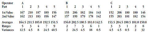
Figure 1: The gasket thickness data. Click here for larger image.The ANOVA approach
Figure 2: Analysis of variance (ANOVA) table for the gasket thickness dataThe AIAG approach
The EMP approach
Figure 4: Interpreting the EMP chart for figure 1
Figure 5: An analysis of main effects (ANOME) chart for operator effect
Figure 6: Comparison of estimates across approachesVariance components for ANOVA
Figure 7: Variance components for ANOVA approachVariance components for EMP approach
Figure 8: Variance components for EMP approachThe AIAG “proportions”
Figure 9: The AIAG “proportions”
Figure 11: Measures of relative utility from the three approachesSummary
Our PROMISE: Quality Digest only displays static ads that never overlay or cover up content. They never get in your way. They are there for you to read, or not.
Quality Digest Discuss
About The Author
Donald J. Wheeler
© 2023 Quality Digest. Copyright on content held by Quality Digest or by individual authors. Contact Quality Digest for reprint information.
“Quality Digest" is a trademark owned by Quality Circle Institute, Inc.
Comments
Flags in the sample parts for GRR
In my study of a GRR, the range of parts you choose for the 10 samples greatly affects the NDC or %GRR. My opinion previously is that I want my gage to be able to determine the difference between good and no good parts, so I have chosen parts to range from out of tolerance low to out of tolerance high. Recently I have seen posts that my sampling should be random according to the current process, but I don't think this tests the gage's ability to determine the difference between good/no good.
What is your opinion of manufacturing the study to include out of tolerance parts?
Thank you,
Ken
(I have posted this on several other threads. I know it is not good form, but please do not delete my account.)
Measurement method acceptability via ANOVA method
In regards to the ANOVA approach, I have only been made aware of using %contribution and its limits (<1% acceptable, 1% to 9% probably acceptable and >9% unacceptable) to determine measurement acceptability. In this article, Dr Wheeler mentioned Estimated ICC as the predominant criteria determining measurement acceptability using the ANOVA method. Even if %contribution is 10%, ICC would be 0.9 which is still a very good correlation, wouldn't it? Did I miss something?
d*2
Thank You
Thought I was losing my mind, seeing phantom bias correction coefficients used by Wheeler that don't match up with the standard charts.