Most shops accept a gauge the same way. They run a gauge repeatability and reproducibility (gauge R&R) study with 10 parts, three appraisers, and three trials. Get a %GRR under 30. File the report and move on. The AIAG criteria are familiar: Under 10% is generally acceptable, 10%–30% may be acceptable, depending on the application, and over 30% is not.

The trouble is what %GRR compares. It divides measurement variation by total variation, and total variation depends on the parts you picked. Choose parts that are spread far apart, and almost any gauge looks good. The number can pass while the gauge is unable to do the job it was bought for.

Here is a worked example, then what to look at alongside %GRR, and how to document the decision so it holds up in an audit.

The study that passes

A shaft diameter is specified at 10.00 mm ± 0.05 mm, so the tolerance is 0.10 mm wide. The gauge is a digital caliper that reads to 0.01 mm. For the study, someone pulls 10 parts from the line and the reject bin so the set covers the full range. The parts run from about 9.94 to 10.06 mm.

The study returns a measurement standard deviation (repeatability and reproducibility combined) of 0.008 mm. The part-to-part standard deviation across the 10 study parts is 0.040 mm.

Total variation is the square root of 0.008 squared plus 0.040 squared, about 0.041 mm. So %GRR is 0.008 divided by 0.041, or 19.6%. The number of distinct categories, 1.41 times the part standard deviation over the measurement standard deviation, comes out at 7. The usual minimum is 5.

By the usual reading, this caliper is acceptable. It sits in the 10%–30% band, and ndc clears the bar. Most reports stop here.

The same gauge against the tolerance

Now ask a different question. How much of the tolerance does the measurement spread consume? The current AIAG manual uses six standard deviations for this. Six times 0.008 is 0.048 mm, which is 48% of a 0.10 mm tolerance. Older worksheets use 5.15 standard deviations and give 41%. Either way, the measurement spread eats close to half of the tolerance.

The study parts didn’t change. The gauge didn’t change. Only the denominator did.

The same gauge against production

Now suppose the process is capable and centered. The real part-to-part standard deviation in production is 0.012 mm, not 0.040 mm. That is a Pp of about 1.39, which most customers would be glad to see.

Recalculate %GRR with the production spread as total variation. The square root of 0.008 squared plus 0.012 squared is about 0.014 mm. %GRR is now 55%. The ndc drops to 2, which means the caliper can sort production parts into roughly two groups. At that point it works as a go/no-go check, not a measuring instrument.

It also distorts what you think you know about the process. Measurement variation adds to process variation, so the observed spread is 0.014 mm rather than 0.012 mm. The same capable process, measured with this caliper, reports a Pp of 1.16 instead of 1.39. Teams chase that gap on the machine when it lives in the gauge.

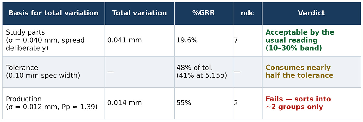
Figure 1: How %GRR changes with what you compare it to. Same gauge, same measurement standard deviation (0.008 mm)—only the denominator changes.

What happens at the limit

Averages hide the cost, so take one part. A shaft that is truly 10.055 mm is 0.005 mm out of tolerance. With a measurement standard deviation of 0.008 mm, a single reading will land at or below 10.050 about 27% of the time. Roughly one in four of those parts gets accepted. A shaft at 10.060 mm still passes about 11% of the time.

If your process runs well centered, few parts sit that close to the limit, and the real-world risk is small. If the process drifts toward one side, or the characteristic is critical, that 27% is the number that matters.

What to look at alongside %GRR

Start with what the gauge is for. If it accepts or rejects product, compare the measurement spread to the tolerance. If it feeds a control chart or a capability study, compare it to the process spread. The AIAG manual allows either basis. The report should say which one was used and why.

Next, check where total variation came from. If it came from the study parts, check that those parts look like production. Parts selected to span the tolerance, or pulled from the reject bin, inflate part variation and make the gauge look better than it is. When you have a reliable historical process standard deviation, calculate %GRR against it as well and report both.

Then look at resolution. A 0.01 mm reading is one-tenth of this tolerance, which meets the usual 10–1 rule. Against the production spread of about 0.072 mm (six times 0.012), it’s closer to one-seventh. Discrimination that’s fine for acceptance can be coarse for process control.

Finally, look at the charts, not just the summary. A range chart with points out of control for one appraiser, or an averages chart where the appraiser lines cross, tells you where the variation is coming from. Those patterns point to technique or fixturing problems that a single percentage never will.

When the gauge falls short

There are four usual responses, and each has a cost.

A better gauge is the clean fix. A micrometer reading to 0.001 mm would likely bring the measurement spread under 10% of this tolerance.

Averaging repeated readings helps less than people expect. Taking the average of n readings cuts the repeatability component by the square root of n. It does nothing for reproducibility, so if appraiser differences dominate, averaging buys little.

Guard banding keeps the gauge and tightens the acceptance limits instead. With limits of 9.966–10.034 mm (two measurement standard deviations inside each specification limit), the shaft at 10.055 mm is accepted about 0.4% of the time instead of 27%. The price is good parts rejected near the limits. In this example, with a centered process, about 1.8% of good parts would fail inspection. Whether that trade is worth it depends on what an escape costs you.

Restricting use is the fourth option. The caliper may be fine for a rough in-process check if final acceptance happens on a better gauge. That’s a legitimate decision as long as it’s written down, and the control plan reflects it.

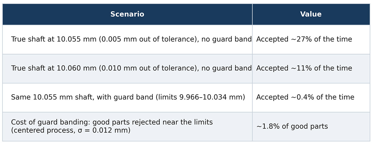
Figure 2: Risk and guard-banding outcomes. Measurement standard deviation = 0.008 mm; specification 10.00 mm ± 0.05 mm.

Writing the decision down

An auditor reading a measurement system analysis (MSA) file wants to know that someone made a decision on purpose. A report that says “%GRR 19.6%, acceptable” invites the question of acceptable for what. For a characteristic on an automotive control plan, IATF 16949, clause 7.1.5.1.1 requires the study, with methods and acceptance criteria that conform to the reference manuals. Other methods need customer approval, with records kept. The AIAG manual treats the 10%–30% band as a judgment based on the application, and says the decision should be approved by the customer. That judgment is exactly what auditors ask to see.

A record that holds up covers six things. First, the characteristic and the gauge. Second, the intended use: product acceptance, process control, or both. Third, the basis for total variation, whether study parts or historical process, with both results if they differ. Fourth, %GRR, the percentage of tolerance, and ndc. Fifth, the decision and any conditions, such as a guard band, a restriction to in-process checks, or a replacement date. Sixth, who approved it and what would trigger a new study, such as a new gauge, a process change, or a customer complaint.

For the caliper above, an honest entry might read: “Acceptable for in-process checks only. %GRR 19.6% on study parts, 55% against production spread; 48% of tolerance. Final acceptance moved to a 0.001 mm micrometer pending its own study. Approved by the quality manager on this date. Restudy on gauge replacement or process change.”

That entry takes 5 minutes to write. It turns a number that could be challenged into a decision that can be defended, and it tells the next person why the caliper isn’t on the final inspection bench.

The short version

%GRR answers one question: How does measurement variation compare with the variation in the parts you studied? Before accepting a gauge, answer two more questions. How does its spread compare with the tolerance it’s judging? And do the study parts look like the parts it will see? When all three answers agree, the gauge is capable. When they don’t, say which one you relied on and why.