When Should We Use Extra Detection Rules?

Using process behavior charts effectively

Published: Monday, October 9, 2017 - 12:03

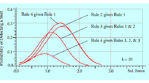
How do extra detection rules work to increase the sensitivity of a process behavior chart? What types of signals do they detect? Which detection rules should be used, and when should they be used in practice? For the answers read on.

In 1931, Walter A. Shewhart gave us the primary detection rule for use with a process behavior chart—look for an assignable cause whenever a single point falls outside the three-sigma limits. In 1946, Eugene L. Grant’s book, Statistical Quality Control (McGraw-Hill Book Co., first edition), gave several additional run tests that could be used to supplement the primary detection rule. However, all of these run tests were concerned with detecting a single type of signal—a long run on either side of the central line. Using multiple detection rules for a single type of signal seemed rather ad-hoc and arbitrary, and so these rules were never very popular. It was not until 1956 and the publication of the Western Electric Statistical Quality Control Handbook that we finally obtained a coherent set of run tests designed to increase the sensitivity of the process behavior chart in a systematic manner. These are the Western Electric Zone Tests found in virtually all of today’s software packages. Then, in 1984 and 1985, Lloyd Nelson gave a list of eight detection rules that he had compiled and used at Nashua Corp. (Seven of these rules came from the Western Electric Statistical Quality Control Handbook.) He published these rules in his column “Technical Aids,” Journal of Quality Technology, v. 16, Oct. 1984, pp. 238–239, and commented on their use in Journal of Quality Technology, v. 17, April 1985. We will consider the rules in Nelson’s list later. 

We will begin by using the Western Electric Zone Tests to examine the effects of additional detection rules upon the sensitivity of the process behavior chart. We do this because we have the power function formulas for these detection rules, and these formulas allow for a rigorous evaluation. While the first 34 of these power function formulas were published by Wheeler in Journal of Quality Technology, v. 15, Oct. 1983, pp. 155–169, Stauffer later expanded this set to 40 formulas. The revised paper “Power Functions for Process Behavior Charts” with all 40 formulas is now available in the SPC Press reading room. Readers interested in the formulas and tables of the power functions as well as the foundation material behind this article are directed to this paper.

Western Electric Zone Tests

Detection rule one: a point outside the three-sigma limits. Whenever a single point falls outside the three-sigma limits look for a dominant assignable cause that has caused your process to change.

Since three-sigma limits will filter out virtually all of the rou­tine variation, any point outside the three-sigma limits is a potential signal. Moreover, the further a point is outside the limits, the stronger the evidence that a change has occurred. False alarms, when they occur, will be rare and will tend to be just barely out­side the limits, so as the number of points outside the limits increases, and as their dis­tance outside the limits increases, we can be confident that the process is indeed being operated in an unpredictable manner.

Detection rule two: a run beyond two sigma. Whenever two out of three succes­sive values are both on the same side of the central line and are both more than two sigma units away from the central line, look for the cause of a small or intermediate shift in the underlying process. 

Detection rule three: a run beyond one sigma. Whenever four out of five succes­sive values are on the same side of the central line and are also more than one sigma unit away from the central line, we should look for the cause of a small shift in the un­derlying process.

Detection rule four: a run about the central line. Whenever eight successive values all fall on the same side of the central line, you should look for the cause of a small but sus­tained shift in the underlying process.

As run tests, detection rules two, three, and four can only be used when the notion of sequence makes sense for your data. They cannot be used with an arbitrary ordering of the data. Moreover, due to the nature of the moving range computation, detection rules two, three, and four should not be used with the moving range portion of an XmR chart. 

To illustrate how detection rules work we use power functions. Power functions show the theoretical probability of detecting a shift vs. the size of an assumed step-function shift. As always, probabilities are limited to fall between 0.0 and 1.0, and for simplicity of representation, the shifts are all expressed in “standard error” units. (For an explanation of standard error see the paper by Wheeler and Stauffer cited earlier.)

To make comparisons between the various detection rules possible we consider the power function at that point where k = 10 “subgroups” have been collected following the shift. While all power functions are theoretical, they serve to approximate how the process behavior chart will function in practice.

Figure 1 shows the power functions for using different combinations of the Western Electric Zone Tests. For simplicity in discussion we shall consider how the various combinations will detect small, intermediate, and large shifts in the process. Shifts in excess of 2.5 standard errors will be called large shifts. Shifts between 1.5 standard errors and 2.5 standard errors will be called intermediate shifts. Shifts smaller than 1.5 standard errors will be called small shifts.

Detection rule one

The first curve on the right in figure 1 shows the power for detection rule one when it is used by itself. Detection rule one will detect a large shift within 10 subgroups at least 39 times out of 40 (probability ≥ 0.975), and it will detect intermediate shifts at least half the time. This means that detection rule one is already highly efficient at detecting shifts that are large enough to be of economic import in a timely manner. We really cannot improve on the performance of detection rule one with regard to large shifts.

Figure 1: The probabilities of detecting shifts with the Western Electric Zone Tests

Detection rules one and two

The second curve from the right shows the power function when rules one and two are used together. The use of rule two makes the power function curve steeper and moves it to the left; this means that smaller shifts are detected with greater probability. With these two rules we can be virtually certain to detect large shifts within 10 subgroups, and we will detect intermediate shifts about four times out of five. Thus, when used with detection rule one, detection rule two increases the sensitivity of the process behavior chart to small and intermediate shifts. By looking at the difference between the first two curves in figure 1 we can obtain a curve that defines the additional power added by the use of detection rule two. This curve is shown in figure 2. 

Figure 2: The additional power gained by using detection rule two with rule one

Differences in theoretical power that are less than 0.05 will hardly be noticed in practice. When we interpret figure 2 in this light we find that rule two is most effective in detecting shifts between 0.5 standard errors and 2.3 standard errors, with the greatest gain in power being centered around shifts of 1.5 standard errors. Thus, rule two principally acts to increase the chance of detecting intermediate and small shifts. Rule two cannot appreciably affect the probability of detecting large shifts because detection rule one will usually get there first.

Detection rules one, two, and three

Returning to figure 1, the third curve from the right shows that the use of rules one, two, and three together will shift the power function curve to the left and slightly increase its steepness. When using rules one, two, and three together we have a probability of at least 94 percent of detecting an intermediate or large shift within 10 subgroups.

Figure 3: The additional power gained by using detection rule three with rules one and two

Figure 3 shows what rule three adds to the use of rules one and two together. Rule three is most effective in detecting shifts between 0.4 standard errors and 1.8 standard errors, with the greatest gain in power being centered around shifts of 1.1 standard errors. Thus, the use of detection rule three in addition to rules one and two principally increases the sensitivity of the process behavior chart to small shifts. It adds nothing to the ability of the chart to detect large shifts, and only slightly increases the ability of the chart to detect the smaller intermediate shifts.

Detection rules one, two, three, and four

Returning to figure 1, the fourth curve from the right shows the power function for rules one, two, three, and four used together. Unlike the second and third curves, we find only a slight shift to the left with this fourth curve. With all four rules the process behavior chart has at least a 96-percent chance of detecting an intermediate, or large, shift (up from 94 percent with rules one, two, and three). When we look at the additional power added by rule four we get the curve in figure 4.

Figure 4: The additional power from detection rule four when used with rules one, two, and three

Figure 4 shows what rule four adds to the use of rules one, two, and three together. With a maximum power increase of 0.086 for shifts of 0.9 standard errors, rule four is effective in detecting shifts of 0.5 to 1.2 standard errors when used with the other three rules. Overall, it adds very, very little to what will have already been found with rules one, two, and three.

So why bother with rule four? There is one practical reason for doing so. Rule four is easy. It is easy to use, it is easy to understand, and it is easy to explain to others. This is why for years most practitioners used only detection rules one and four. No extra computations were needed, Long runs and points outside the limits were, and still are, easy to see when you look at the chart. And since looking at the chart is a prerequisite for the effective use of any process behavior chart, we need to consider what happens when detection rules one and four are used together to the exclusion of all other detection rules

Detection rules one and four

When we compute the power function for the use of detection rules one and four together we get the curve shown on the left in figure 5. There we see that, within 10 subgroups, large shifts are virtually certain of being detected, and intermediate shifts will be detected about four times out of five.

Figure 5: The power function for detection rules one and four

As before the difference between the two curves in figure 5 will show the additional power obtained by using detection rule four in addition to detection rule one. Surprisingly, the additional power obtained from using rule four as the first additional rule effectively dominates that of the other rules, as may be seen in figure 6. Rule four, when used with detection rule one, increases the sensitivity of the chart to small and intermediate shifts very much like the addition of rule two did earlier.

Thus, on the one hand, detection rule four can provide a substantial boost to the ability of a process behavior chart to detect intermediate and small shifts when it is used with detection rule one. On the other hand, detection rule four will only provide a minimal boost to the power of a process behavior chart when it is used with detection rules one, two, and three. This means that the ability of a detection rule to increase the sensitivity of a process behavior chart will depend upon how many other detection rules are also being used. 

Figure 6: The additional power functions compared

This dependence upon the number of rules being used makes the development of power functions for all the possible combinations of detection rules impracticable. (Just developing the formulas for the power functions in figure 1 required the enumeration of 212,576 combinations of points that resulted in the detection of a shift!) However, there are some generalizations that can be made based on the known power functions given here. We begin with figure 5 above.

Detection rules one and four together are virtually certain to detect large shifts, and have about a 79-percent chance of detecting intermediate shifts. This leaves very little for additional detection rules to do. No matter how many additional detection rules we might use, about all that we can hope to accomplish with additional rules will be to detect some small shifts. Both this tendency toward detecting smaller shifts and the diminishing return associated with the use of additional detection rules can be seen in the way the various curves of figure 6 shift to the left and shrink in size as more rules are used.

Nelson’s detection rules

Since Lloyd Nelson’s list of eight detection rules are used in several popular software programs, we will consider the effects of using these detection rules. 

Nelson’s rule one: Nelson’s first rule is Western Electric rule one: a single point outside three sigma limits is interpreted as a signal of a substantial process shift. This is the detection rule Shewhart gave us. It is the standard, it is our primary detection rule, and it has stood the test of time. As seen in figure 1, within 10 subgroups, this rule will single-handedly detect virtually all large shifts and the larger intermediate shifts as well. Shewhart, Nelson, and everyone else who has ever written about SPC recommend starting with rule one only. 

Recommendation: Always use rule one (with three sigma limits).

Nelson’s rule two: Nelson’s rule two is a conservative form of Western Electric rule four. Nelson uses “nine in a row” rather than eight in a row on either side of the central line. Figure 7 shows the power function for using Nelson’s rules one and two together versus using Western Electric rules one and four.

Figure 7: Comparing Nelson’s rules one and two with detection rules one and four

While Nelson’s rules one and two have virtually the same power as the Western Electric Rules one and four, they have about half the risk of a false alarm. This was the reason Nelson chose nine in a row rather than eight in a row. Figure 7 shows that it was a good call. Nelson recommended using rule two in addition to rule one when more sensitivity is desired. 

Recommendation: Use Nelson’s rules one and two when seeking increased sensitivity to intermediate process shifts. As long as rule one is giving multiple signals of process changes the use of Nelson’s rule two is unnecessary.

Nelson’s rule three: Nelson’s rule three is “six points in a row steadily increasing or decreasing.” This rule has been examined in two separate studies and has been found to be of little value. Robert B. Davis and William H. Woodall note that Nelson’s rule three “is of virtually no help in the detection of drifts in the process mean if other runs rules are already being used.” and it “is not performing the task which it was supposedly designed to perform.” (Journal of Quality Technology, v. 20, Oct. 1988, pp. 260–262.) Esteban Walker, John W. Philpot, and James Clement note that “Among the eight rules considered, rule 3 seems to contribute substantially to the high [false alarm] risks.” (Journal of Quality Technology, v. 23, July 1991, pp. 247–252.) Thus, according to both of these studies, Nelson’s rule three adds more to the false alarm rate than it does to the power of the process behavior chart. 

One easy way to understand why Nelson’s rule three does not work is to recall that the average distance between two successive averages or individual values is d2 = 1.128 standard errors. Thus, even when the process is not changing, the average spread of a “run of six” will be something like 5.6 standard errors. This will make it difficult to fit a ”run of six” within limits that are only six standard errors wide.

Figure 8: Why runs-up-and-down rules don’t work

So, unless the first point of the run of six is more than 2.6 sigma away from the central line, (an event that has a probability of less than 0.005 of happening by chance) the last point of the run of six is very likely to fall outside the three sigma limits. Because of this, before Nelson’s rule three will detect a trend, rule one is very likely to have already detected the change in the process. 

While Nelson recommended using rule three when more sensitivity was needed, both of the articles cited found that it did not add to the sensitivity of the process behavior chart. Tests for runs-up-and-down were created for use with finite data sets. In this context, and in the absence of other detection rules, they can be useful in identifying changes and trends within the data. But once we have computed three-sigma limits and are using rule one, the runs-up-and-down tests become redundant.

Recommendation: The best modern practice is to completely avoid using Nelson’s rule three and all other runs-up-and-down tests as well. Rule one will get there first in most cases.

Nelson’s rule four: Nelson’s rule four is “fourteen points in a row alternating up and down.” This is generally the result of a mixture of two different processes on the same chart. It was discussed and illustrated in Wheeler’s “Autocorrelated Data” (Quality Digest, Aug. 7, 2017). Nelson recommended using this rule when more sensitivity was needed. However, this rule comes from the Western Electric Handbook where it was intended for use when setting up a chart as a way to detect mixtures. It looks for a specific pattern rather than adding sensitivity to a process shift.

Recommendation: Nelson’s rule four is useful when first setting up a process behavior chart, but it has little utility once the chart is being used in production.

Nelson’s rules five and six: Nelson’s rule five is Western Electric rule two. Nelson’s rule six is Western Electric rule three. The behavior of these two rules has been examined above. As shown in figure 1, when these two rules are used with rule one we essentially achieve the maximum possible power for a process behavior chart. The use of additional detection rules can only pump up the risk of a false alarm while increasing sensitivity to small shifts. Nelson recommended using these rules in an “engineering study” to “increase the sensitivity to changes.”

Recommendation: Nelson’s rules five and six can be used with his rule one, or even with his rules one and two, to essentially achieve the maximum power possible from a process behavior chart. However, the increased sensitivity to small and intermediate shifts provided by rules five and six will be of little use as long as rule one continues to give evidence of large process shifts.

Nelson’s rule seven: Nelson’s rule seven is for “hugging the central line”—fifteen points in a row all within one sigma of the central line. This is most often the result of stratified subgroups where each subgroup contains data from two or more different production processes. While this phenomenon may be found on average charts, it will often show up first on the range chart. (Since this rule looks for stratified subgroups it is not appropriate for use with an XmR chart where the subgroup size is one.)

This rule is one of the pattern detection guidelines from Western Electric that can be useful during the baseline phase of creating an average and range chart. By warning that the subgrouping may not be rational, it can help to avoid the creation of a useless chart. However, once the subgroups have been organized in a rational manner, this rule turns out to be of little use during production. Nelson did not include this rule in the list of rules for routine use.

Recommendation: We concur with Nelson, rule seven is useful when first setting up an average and range chart, but it has little utility once the chart is being used in production.

Nelson’s rule eight: Nelson’s rule eight is essentially the converse of rule seven. Investigate whenever eight successive values are all more than one-sigma away from the central line. This rule is a generalized version of Nelson’s rule four where the data reflect two different processes. Here the data might not alternate between the two different processes in succession, but they are definitely stratified between the “subgroups” and are likely to yield a bimodal histogram. Like Nelson’s rules four and seven, this rule is essentially a pattern detection guideline that can be useful during the baseline phase of creating a process behavior chart. However, the basic rules (Western Electric rules one, two, or three) are very likely to detect this problem before Nelson’s rule eight works. Nelson did not include this rule in the list of rules for routine use.

Recommendation: We concur with Nelson, rule eight is useful when first setting up a process behavior chart, but it has little utility once the chart is being used in production.

Using additional detection rules

Rule one is sufficient for most cases. 

Using rule one with Nelson’s rule two will usually detect more signals than you will have time to investigate. 

However, the authors have heard some statisticians suggest “If it is there, why not use it?” So what would happen if we added additional detection rules to the mix? Figure 9 gives a clue. Whenever we add a detection rule it has the effect of moving the power function curve to the left. However, as we add more rules these incremental improvements in power become smaller. We see this in how the curves get closer together as they move to the left. Thus, the additional power gained by using an extra detection rule will never be as great as it might appear to be when that detection rule is considered by itself.

Moreover, there is a limit to how much information may be extracted from a given amount of data. As the power function approaches this limit the only way that a detection rule has of moving the power curve to the left is by allowing the beginning point of the curve to shift upward. This can also be seen in figure 9. 

Figure 9: The effect of using extra detection rules

Since the beginning point of each power curve is the theoretical false alarm probability for that curve, we find that there is a diminishing return for the use of additional detection rules. As more rules are used the risk of a false alarm will increase while the additional power gained by adding those rules will dwindle. 

For the eight combinations of detection rules listed in figure 9, figure 10 summarizes the minimum power for detecting large and intermediate shifts within 10 subgroups of when they occur. It also lists the false alarm probabilities over 10 consecutive subgroups. When we recall that small differences in theoretical power are unlikely to be noticed in practice, we can summarize the lessons of figures 9 and 10. 

Once we use rule one, all of the remaining, undetected shifts will be either intermediate or small shifts. 

Once we use an “acceptable” combination from figure 10, most of the remaining, undetected shifts will be small shifts.

Once we use a “max power” combination from figure 10, all of the remaining undetected shifts will be small shifts. 

Since, by definition intermediate shifts will have less economic impact than larger shifts, the use of extra detection rules will inevitably involve a search for shifts of decreasing economic importance. Thus, when you use extra detection rules you are unavoidably risking an increased chance of a false alarm, and using rules that have less and less power, while searching for shifts that are relatively unimportant. A better formula for increasing futility could never be devised.

Figure 10: Detection rule recommendations

Using software

As if the proliferation of detection rules was not already enough to overwhelm the user with choices and the resulting false alarms, we live in the age of do-it-yourself statistics where each person gets to create their own detection rules by tweaking the rules given above. The software allows you to choose something other than three sigma limits for Nelson’s rule one, something other than 9 in a row for Nelson’s rule two, etc. To illustrate the point from the preceding section, consider what happens when rule one is naively changed to use two sigma limits. 

Figure 11 shows that modifying rule one to use two-sigma limits, and using that modified rule alone, will not appreciably increase the probability of detecting intermediate or large shifts over what can be accomplished with the other detection rules. While this modified rule will increase the chances of detecting small shifts, it does so by greatly increasing the risk of false alarms.

Figure 11: User-modified detection rules can result in excess false alarms

To have a discriminating technique we want a power function that starts low and increases rapidly. The curve for two sigma limits does not start low and has an unacceptable risk of false alarms. For this reason two sigma limits are inappropriate for a sequential procedure. Since the traditional detection rules at least strike a partial balance between the alternatives of power and false alarms, users should always avoid making up their own detection rules. Believe us when we say that when it comes to probability and statistics, you always know much less than you think you know.

Summary

The search for any and all process shifts is not recommended. According to Shewhart, “… we must use limits such that through their use we will not waste too much time looking unnecessarily for trouble.” and “… the limits on all the statistics should be cho­sen so that the probability of looking for trouble when any one of the chosen statistics falls outside its own limits is economic.” (Economic Control of Quality of Manufactured Product, pages 148 and 277.)

Process behavior charts are all about knowing when it is economical to intervene and when it is economical to leave the process alone. To this end detection rule one has proven to be sufficient in most cases. Rule one strikes a balance between the consequences of either getting a false alarm or missing a signal of economic importance. Using additional detection rules shifts this balance. It skews the balance it toward more false alarms in order to find smaller signals. This is generally unnecessary and should not be done without careful consideration of the situation at hand. Additional detection rules should very definitely not be used just because the software allows you to do so.

Rule one has been the key to process improvement for more than 90 years. Use it and learn about the dominant assignable causes affecting your process. In practice, rule one will usually generate all the signals that most people can realistically investigate. And since investigation of signals is the key to the effec­tive use of process behavior charts, you should be careful about introducing additional detec­tion rules. The charts are intended to be a basis for action, rather than an unending nag which you must ignore in self defense.

About The Authors

Donald J. Wheeler

Dr. Wheeler is a fellow of both the American Statistical Association and the American Society for Quality who has taught more than 1,000 seminars in 17 countries on six continents. He welcomes your questions; you can contact him at djwheeler@spcpress.com.

 

Rip Stauffer

Rip Stauffer uses his extensive experience in total quality and Six Sigma to educate and counsel at all career levels with specific experience in government, manufacturing, medical devices, financial services, and healthcare organizations. A senior consultant at MSI, and CEO of Woodside Quality LLC, Stauffer is an ASQ senior member and statistics division member, a certified quality engineer, a manager of quality and organizational excellence, and a Six Sigma Black Belt and Master Black Belt. He also is an adjunct faculty member at Walden University, teaching graduate and undergraduate business statistics courses and international business courses.