Converting Capabilities

What difference does the probability model make?

Published: Monday, October 3, 2022 - 12:03

Last month we found that capability and performance indexes have no inherent preference for one probability model over another. However, whenever we seek to convert these indexes into fractions of nonconforming product, we have to make use of some probability model. Here, we’ll look at the role played by probability models when making these conversions.

Many people have been taught that the first step in the statistical inquisition of their data is to fit some probability model to the histogram. Here we’ll begin with the 250 values shown in figure 1. These values have an average of 7.4 and a standard deviation statistic of 5.2.

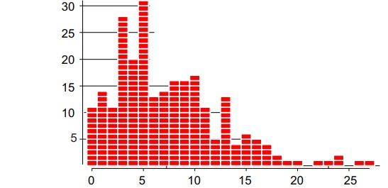
Figure 1: 250 observations from one process

Clearly these data have a skewed histogram with a barrier or boundary condition on the left. As may be seen in figure 2, a normal distribution having a mean of 7.4 and a standard deviation of 5.2 isn’t going to provide a very good fit to this histogram. It under-represents the values from 0 to 5, and overrepresents both the negative values and those values from 6 to 14.

Figure 2: Data with fitted normal model

Next we consider the statistician’s favorite skewed model, the lognormal distribution. These 250 data have a median value of 6, so the lognormal distribution with alpha = 6 and beta = 0.65 has a median of 6.0 and a mean of 7.4. This lognormal (6.0, 0.65) model does a reasonable job of “fitting” this histogram. However, it doesn’t allow for the abundance of 0 and 1 values found in these data.

Figure 3: Data with fitted lognormal model

So, perhaps another distribution will do a better. job. A gamma distribution with alpha = 2 and beta = 2 (also known as a Chi-square distribution with four degrees of freedom) has a mean of 4 and a standard deviation of 2.828. When we stretch this distribution out 185% we get a distribution with a mean of 7.4 and a standard deviation of 5.23, which results in the fitted model shown in figure 4. This model does a better job in terms of allowing for the values at 1 than did the lognormal model.

Figure 4: Data with fitted a stretched gamma model

Finally we consider the favorite models of reliability theory, the Weibull distributions. A Weibull distribution with alpha = 1.5 and beta = 8.2 will have an average of 7.4 and a standard deviation of 5.03. This probability model does a good job at 0 and 1 and also for 8 and above, but it has a broader and flatter mound than the histogram.

Figure 5: Data with fitted Weibull model

For reasons that will become clear, we’ll ignore the question of how to choose one of these probability models over the others. Here we’ll use all four of these fitted models to convert various values of an upper specification limit into estimated fractions nonconforming.

Figure 6: The four models considered

Since these data come in one-unit increments, we’ll consider upper specification limits starting at 12.5 and continuing on up to 35.5. For each of these USL values, we’ll compute the corresponding estimated fraction nonconforming using each of the four models in figure 6.

The horizontal axis in figure 7 lists the USL values up to 23.5 and their corresponding Ppk values (from 0.33 to 1.03). The vertical axis lists the percent nonconforming. Each of the four fitted models is represented by a separate curve that shows the estimated percent nonconforming as a function of the USL values.

Figure 7: Percent nonconforming

On the left, at USL = 12.5, the normal distribution gives the largest estimated fraction nonconforming. But by the time the USL gets to 14.5 (Ppk = 0.46) and beyond, it’s the skewed models that give the larger estimates of the fraction nonconforming.

Figure 8 shows the estimated fractions nonconforming in parts per thousand for Ppk values from 1.10 up to 1.80. Here, the skewed models begin to yield estimated fractions nonconforming that differ by up to 6 fold.

Figure 8: Parts per thousand nonconforming

The differences in figure 8 are relatively substantial, which makes it seem like our choice of probability model is important. However, before we get too concerned about how the estimates in figures 7 and 8 differ, we need to think about how they are alike. And to do this we need to have a way to construct error bars for our estimates.

Error bars for fractions nonconforming

Error bars are a common part of the way scientific and technical estimates are reported. So how can we construct error bars for the estimates above? In statistical jargon, error bars are often known as confidence intervals, or more correctly, interval estimates. Since this whole exercise begins with a collection of data, and since an estimate cannot be better than the data upon which it’s based, we must begin with the inherent uncertainty contained in the data themselves.

The empirical estimate of the fraction nonconforming is the simple ratio known as the binomial point estimate, p.

For example, if the USL is 12.5, then figure 1 shows 42 out of 250 to be nonconforming and our empirical estimate of the fraction nonconforming is:

This empirical estimate of 16.8 percent is consistent with the starting points for the four curves in figure 7. But how much uncertainty is inherent in this value of 16.8 percent?

Since 2003, the preferred way to characterize the uncertainty of a point binomial estimate is to use an Agresti-Coull interval estimate. The Agresti-Coull interval estimate is centered on the Wilson point estimate. This is done to take into account the asymmetry in the error bars that occurs as the proportions get close to zero or 1.00. The Wilson point estimate for 95-percent error bars may be found by adding two conforming and two nonconforming items to the counts in the binomial point estimate. Here we would have:

Once we have this value, the 95% Agresti-Coull interval estimate is found by computing:

So the empirical estimate of 16.8 percent has error bars that go down to 12.7 percent and up to 22.0 percent. This inherent uncertainty of the empirical estimate is a property of the data. This is all these data will support. No assumption we can make can reduce this inherent uncertainty.

Yet when we choose a probability model to use in estimating a fraction nonconforming, we’re making an unverifiable assumption. The uncertainty of this assumption can only add to the inherent uncertainty contained in the data. Thus, all model-based estimates must be interpreted relative to the error bars for the empirical estimates. Figure 9 lists the 95 percent error bar values along with the model-based estimates for USL values between 12.6 and 35.5.

Figure 9: Estimated fractions nonconforming and 95-percent error bars

The error bars only change value when the number of nonconforming items changes, so we show them as step functions in figure 10.

The skewed models all provide a reasonable fit to our histogram, and the three curves for these models all fall within the error bars. They’re all consistent with the empirical estimates. So, while the different models give different estimates, the uncertainty in these estimates is so great that, at any given value of Ppk, the various models are essentially estimating the same thing! Even when the lognormal model gives estimates that are three, four or five times as large as the estimates from the Weibull model, these different estimates all have so much uncertainty attached that we simply cannot interpret them as being different.

Figure 10: 95-percent error bars for estimated fractions nonconforming

The ultimate uncertainty

Every histogram has a minimum and a maximum. Once we go beyond either of these extremes, we have left the data behind. So what does the absence of data tell us about the underlying process? The answer lies in the error bars that correspond to an observed number nonconforming of zero.

In figure 1, the maximum observed value is 27. As the USL value continues to increase beyond 27.5, the model-based estimates in figure 9 continue to shrink as these estimates rely upon the increasingly infinitesimal areas in the extreme tails of the probability models.

However, even though Ppk may increase as the specifications get wider, once we go beyond the end of the histogram the error bars remain fixed. These ultimate error bars depend only upon the number of data in the histogram. For 250 data we have ultimate error bars of 0.0 percent to 1.9 percent. In the absence of any observed nonconforming items, this is as precise as 250 data will allow the estimate to be.

So while the use of model-based estimates will allow us to estimate the fraction nonconforming out beyond the end of the histogram, and while these estimates can be computed out to many decimal places, they will all have a fixed level of uncertainty.

Moreover, this fixed level of uncertainty can be much greater than the estimates themselves. For example, in figure 9, when the USL is 35.5, the skewed models estimate 0.36 percent, 0.09 percent, and 0.03 percent nonconforming. Yet all three of these estimates all have 95 percent error bars of 0.0 percent to 1.9 percent nonconforming.

Thus, the number of data in our histogram will determine the ultimate 95 percent error bars. Figure 11 shows these ultimate 95% upper error bar values for different amounts of data.

Figure 11: Ultimate 95-percent upper error bars

The values in figure 11 are the 95 percent upper bound for the Agresti-Coull interval estimate for the fraction nonconforming for specifications where there are zero observed nonconforming values in a histogram consisting of n values.

So, if you use a histogram of 400 data to fit a model, and if that model-based estimate of the fraction nonconforming turns out to be 3 or 4 parts per million, your 95 percent upper error bar for this estimate is going to be 1.2 percent, or 12.000 parts per million!

To get estimates of tail area probabilities with an ultimate 95-percent upper error bar as small as one part per thousand, you will need to use at least 5000 data.

This means that virtually all claims of parts per million levels of nonconformity are bogus. These estimates may be computed exactly and correctly, but they’re nothing more than an artifact of the probability model selected. Those who use parts per million estimates based on probability models have simply been seduced by computations that are devoid of content because they have been taken out of context. Such estimates have no contact with the underlying data or the process it represents.

No assumption we make can reduce the inherent uncertainty of the data themselves. Our assumed probability models may allow for the computation of infinitesimal areas in the extreme tails, but it is the height of naiveté to believe such computations represent reality.

Lessons of the exercise

Our statistical inquisition began with fitting models to our histogram. The skewness of our histogram led us to consider three different skewed probability models. These three models gave us estimates for the fraction nonconforming that appeared to be different. Yet when we took their inherent uncertainty into account, the estimates were all indistinguishable. Since this game of fitting various and sundry probability models to the data is most often the result of a skewed histogram, we need to conclude by considering how histograms get skewed.

The usual source of skewness

Before we can ever successfully fit a model to our data, the data will need to be homogeneous. And the primary tool for checking a data set for homogeneity is the process behavior chart. When we use the time-order sequence of the 250 data in figure 1 and arrange them into subgroups of size 5, we get the average chart of figure 12.

Figure 12: Average chart for data of figure 1

With five points above the upper average limit and the two runs on the low side, we have solid evidence that this process was moving around while these data were obtained. The skewness is an artifact of the process changes, rather than being a property of the process itself. While the descriptive statistics describe the past, they cannot be said to provide valid estimates for the parameters of any probability model. Thus all four models used above are in error, and none are useful for predicting the future process behavior.

Probability models are built on the assumption that the data can be thought of as observations from a set of random variables that are independent and identically distributed. When the data aren’t homogeneous, this assumption is patently untrue and the notion that the data can be represented by a probability model evaporates.

Since most processes are operated unpredictably, the most common source of a skewed histogram is the process going on walkabout. When this is the case it is a mistake to fit a probability model to the histogram, since the histogram is a mixture of data from a process with multiple personalities.

Summary

If your process is operated predictably, then empirical estimates of the fraction nonconforming allow for prediction, and estimates obtained from any appropriate model will mimic the empirical estimates.

If your process has been operated unpredictably, then the empirical estimate of the fraction nonconforming will describe the past. But here the past will offer no basis for predicting the future. Fitting a probability model can only mislead, and so is to be avoided.

In the end, which probability model you may fit to your data hardly matters. It is an exercise that serves no practical purpose. Empirical estimates, and their uncertainties, will always trump any model-based estimate. And when your process has been operated unpredictably, no probability model has any integrity or validity.

Finally, figure 11 shows that no probability model will ever provide meaningful estimates beyond the parts per thousand level. If you have fewer than 5000 data, the uncertainty of any estimate will exceed one part per thousand. When you have more data, the process will almost certainly be unpredictable and no one probability model will be appropriate.

The numerically naive think that two numbers that are not the same are different. But statistics teaches us that two numbers that are different may actually be the same.

About The Author

Donald J. Wheeler

Dr. Wheeler is a fellow of both the American Statistical Association and the American Society for Quality who has taught more than 1,000 seminars in 17 countries on six continents. He welcomes your questions; you can contact him at djwheeler@spcpress.com.