Cost for QD employees to rent an apartment in Chico, CA. $1,200/month. Please turn off your ad blocker in Quality Digest
Our landlords thank you.
Donald J. Wheeler
Published: Monday, February 6, 2023 - 13:03 The shape parameters for a probability model are called skewness and kurtosis. While skewness at least sounds like something we might understand, kurtosis simply sounds like jargon. Here we’ll use some examples to visualize just what happens to a probability model as kurtosis increases. Then we’ll combine the visible effects of both skewness and kurtosis to see how they combine to “shape” probability models Last month, we found that while an increase in positive skewness measures a nearly invisible increase in the area of the upper tail, it has two visible manifestations. Specifically, these are a substantially shorter lower tail and an appreciable shift of the mode to the left. Figure 1 summarizes these results for the three comparisons made. Figure 1 shows what happens when we hold the kurtosis constant and increase the skewness. In the comparisons that follow, we’ll look at what happens when we increase the kurtosis while holding the skewness constant. While kurtosis is based on a Greek word usually translated as “arched,” “peaked,” or “convex,” it can be hard to see how to apply these adjectives to the complex shapes of probability models. The first reason for this difficulty is that skewness and kurtosis are defined in terms of standardized variables. So, as with skewness, we must use standardized probability models to discover the visual effects of kurtosis. In an earlier column (“So What Are Skewness and Kurtosis?” Quality Digest, Sept. 7, 2021) I demonstrated how the formula for kurtosis emphasizes the extreme values in the tails of a probability model. Since these extreme values will tend to be part of the invisible portion of the probability model, it has always been difficult to see the direct effects of increasing kurtosis. Computationally, kurtosis depends upon what happens out of sight. However, like skewness, kurtosis has some visible effects. The standardized Burr distributions in Figure 2 are very nearly symmetric with kurtosis values of 2.8 and 3.9. We can change the first distribution into the second by shifting around just 54 parts per thousand of the area under the curve. From the lower shoulder between -2.3 and –0.7 we will need to shift 22 ppt up into the central region between -0.7 and +0.7. Also from the lower shoulder between -2.3 and –0.7 we will need to shift 6 ppt down into the lower tail below -2.3. Of these 6 ppt going into the lower tail, 3 will be shifted down below –3.0. From the upper shoulder between +0.7 and +2.4 we will need to shift 22 ppt down into the central region between -0.7 and +0.7. Also, from the upper shoulder between +0.7 and +2.4 we will need to shift 4 ppt up into the upper tail above +2.4. Of these 4 ppt going into the upper tail, 3 will be shifted up above +3.0. (This asymmetric shift into the tails does slightly increase the skewness of the second distribution.) Of the 54 ppt that were shifted, 44 ppt went into the central mound and only 10 ppt went into the tails. The 44 ppt shifted inward compensate for the increased rotational inertia of the 10 ppt shifted outward. They keep the mean at zero, the standard deviation at 1, and the skewness near zero, while allowing the kurtosis to change from 2.80 to 3.90 So what is the impact of increasing kurtosis? Kurtosis is heavily dependent upon the extreme tails, with 52 percent and 67 percent respectively coming from the areas beyond ±3.0 here. Kurtosis directly measures the extent to which the tails get heavier, yet the changes in the tails are almost invisible in Figure 3. The 44 ppt moving from the shoulders to the central region result in the visible effect of the increase in kurtosis. In the region near the mean of zero, the curve of the probability model becomes more “arched” as kurtosis increases. This comparison will use two Burr distributions having a skewness of 0.84 and kurtosis values of 3.9 and 6.0. These distributions are near the extremes of possible kurtosis for Burr distributions with this skewness. To change the first distribution of Figure 4 into the second, a total of 95 parts per thousand need to be shifted around. Because of the skewness of these models, I let the flow of area define the “shoulders” of the distributions. The regions that lost area as the kurtosis increased are the “shoulders” used here. From the lower shoulder between -1.7 and –0.6 we will need to shift 46 ppt up into the central region between -0.6 and +0.9. Also from the lower shoulder between -1.7 and –0.6 we will need to shift 26 ppt down into the lower tail below -1.7. Of these 26 ppt going into the lower tail, only 1 will be shifted down below –3.0 From the upper shoulder between +0.9 and +3.0 we will need to shift 21 ppt down into the central region between -0.6 and +0.9. Also from the upper shoulder between +0.9 and +3.0 we will need to shift 2 ppt up into the region above +4.0. Of the 95 ppt that were shifted, 67 ppt went into the central mound and 28 ppt went into the tails. The 67 ppt shifted inward compensate for the increased rotational inertia of the 28 ppt shifted outward. They keep the mean at zero, the standard deviation at 1, and the skewness at 0.84, while allowing the kurtosis to change from 3.90 to 6.00 So what is the visual impact of increasing kurtosis for these skewed distributions? While 56 percent and 77 percent of these kurtosis values come from the regions beyond ±3.0, the difference between the upper tails is invisible in Figure 5. Here, kurtosis basically tracks how the weight of the short tail increased. The visible manifestations of the increase in kurtosis for these positively skewed distributions are the growth in the area of the lower tail and a shift in the mode toward the mean. Because of the shift towards the mean the curve for the probability model becomes more “arched” in the region near the mean of zero. This comparison will use two Burr distributions having a skewness of 1.41 and kurtosis values of 6.0 and 10.0. These distributions are near the extremes of possible kurtosis for Burr distributions having this skewness. To change the first distribution of Figure 6 into the second, a total of 130 parts per thousand need to be shifted around. Because of the large skewness values, the upper region that loses area, our “upper shoulder,” expands to include most of the upper tail. From the lower shoulder between -1.3 and –0.3 we will need to shift 57 ppt up into the central region between -0.3 and +1.2. Also from the lower shoulder between -1.3 and –0.3 we will need to shift 57 ppt down into the lower tail between –1.3 and –3.0. From the upper shoulder between +1.2 and +4.0 we will need to shift 16 ppt down into the central region between -0.3 and +1.2. Of the 130 ppt that were shifted, 73 ppt went into the central mound and 57 ppt went into the lower tail. The 73 ppt shifted inward compensate for the increased rotational inertia of the 57 ppt shifted into the lower tail. They keep the mean at zero, the standard deviation at 1, and the skewness at 1.41 while allowing the kurtosis to change from 6.00 to 10.00 So what is the visual impact of increasing kurtosis with these heavily skewed distributions? The differences in the upper tail are nearly invisible. The visible manifestations of this increase in kurtosis are the increasing area of the lower tail and the shift of the mode toward the mean of zero. This latter effect causes the curve for the distribution to become more “arched” in the region near zero. Kurtosis is heavily dependent upon the extreme tails of a probability model. But the severe limitations on the areas that can exist in the extreme tails makes the direct effects of changes in both skewness and kurtosis virtually invisible. When we increase kurtosis while holding skewness fixed, any standardized distribution will have an increased arch in the neighborhood of the mean of zero. It is this increased arch that gives us a clue as to why the standardized fourth central moment was named “kurtosis.” When working with skewed probability models, the increased arch will also be accompanied by two other visible effects of increased kurtosis. These are an increase in the area in the short tail and a shift of the mode back toward the mean. As the kurtosis increases, the probability model will look less skewed even though the skewness remains unchanged. Thus, the visible effects of increased kurtosis are contrary to the visible effects of increased positive skewness summarized in Figure 1. So, increased skewness and increased kurtosis have contrary effects on the shape of the distribution. This tug-of-war is just one of the reasons the shape parameters are hard to describe. Which parameter will win out? In the examples used last month, a total area of 514 ppt had to be shifted around to change the skewness. In the examples here, using the same distributions, a total area of 279 ppt had to be shifted to change the kurtosis. Thus, in general, changes in skewness will involve larger shifts in area, and the effects of skewness will dominate over those of kurtosis. So what is the use of the skewness and kurtosis parameters? While the mean and variance of a distribution are primary characteristics of a probability model, skewness and kurtosis are secondary characteristics for the standardized version of that model. The mean and variance describe location and dispersion and will have physical units attached. Skewness and kurtosis characterize the extreme tails of a model and are pure numbers that never have any physical units attached. They are purely theoretical values that allow us to define the similarity or disparity of different models. The shape parameters allow us to organize the various probability models on the shape characterization plane, and thereby to see how different families of probability models are related to one another. However, except for this one theoretical use, the skewness and kurtosis parameters are of little value. Now you know more about shape parameters than you ever wanted to know. You have seen how skewness and kurtosis affect the shape of a probability model, and you have discovered why it is so hard to use these shape parameters in any practical way. When the fundamental meanings behave in a contrary way, practical interpretations fly out the window. Virtually all of the useful information that can be obtained from numerical summaries of the data is found in the statistics for location and dispersion. After location and dispersion, further computations simply chase the noise in your data. This is why skewness and kurtosis statistics have no role to play in the analysis of data. While we all have software that computes the skewness and kurtosis statistics, these values have no practical use in describing or analyzing our data. The problem is that these shape statistics are heavily dependent upon the third and fourth powers of the most extreme deviations from the average. This dependence creates a volatility that makes the statistics useless in practice—they vary so much that they contain no useful information about either the data or the process from which the data were obtained. So, if in the past, for whatever reason, you have simply ignored the shape statistics provided by your software, then keep it up. If you are currently trying to make use of the shape statistics, give it up. When you stop hitting your head against the wall, you will not only feel better but your analysis will be more robust, more sensible, and more appropriate. For the formulas needed to verify these results, see last month’s column. Quality Digest does not charge readers for its content. We believe that industry news is important for you to do your job, and Quality Digest supports businesses of all types. However, someone has to pay for this content. And that’s where advertising comes in. Most people consider ads a nuisance, but they do serve a useful function besides allowing media companies to stay afloat. They keep you aware of new products and services relevant to your industry. All ads in Quality Digest apply directly to products and services that most of our readers need. You won’t see automobile or health supplement ads. So please consider turning off your ad blocker for our site. Thanks, Dr. Wheeler is a fellow of both the American Statistical Association and the American Society for Quality who has taught more than 1,000 seminars in 17 countries on six continents. He welcomes your questions; you can contact him at djwheeler@spcpress.com. Kurtosis Visualized
No one really understands kurtosis. Here’s why.
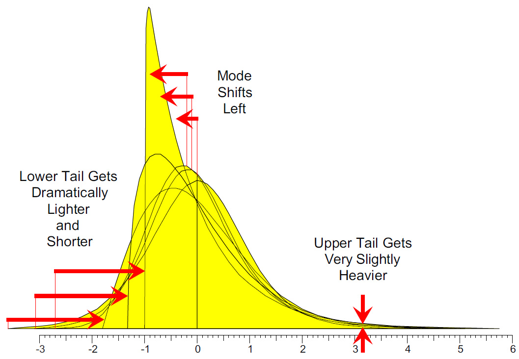
Figure 1: Effects of increasing positive skewness while holding kurtosis constantComparison 1: Kurtosis changes from 2.8 to 3.9
Figure 2: Changing kurtosis from 2.8 to 3.9
Figure 3: Effect of changing kurtosis from 2.8 to 3.9Comparison 2: Kurtosis changes from 3.9 to 6.0
Figure 4: Changing kurtosis from 3.90 to 6.00
Figure 5: Effect of changing kurtosis from 3.9 to 6.0Comparison 3: Kurtosis changes from 6.0 to 10.0
Figure 6: Changing kurtosis from 6.00 to 10.00
Figure 7: Effect of changing kurtosis from 6.0 to 10.0Summary
Figure 8: Effects of increased kurtosis with constant positive skewnessRecommendation
Appendix
Figure 9: Burr distributions used
Our PROMISE: Quality Digest only displays static ads that never overlay or cover up content. They never get in your way. They are there for you to read, or not.
Quality Digest Discuss
About The Author
Donald J. Wheeler
© 2023 Quality Digest. Copyright on content held by Quality Digest or by individual authors. Contact Quality Digest for reprint information.
“Quality Digest" is a trademark owned by Quality Circle Institute, Inc.
Comments
Excellent
I love how Dr. Wheeler explains the mathematical details for those who care about such things, but boils it all down to what 99.9% of all practitioners need to know in a just few key sentences using simple language at the end.
Dr. Wheeler is a treasure as he is one of the few who tries to simplify things instead of complicate them unnecessarily.