Capability indexes allow us to characterize the relationship between the process potential and the specifications. Performance indexes characterize the past performance relative to the specifications. Yet, in practice, we seek to make sense of these index numbers by converting them into other quantities such as the fraction nonconforming or the parts per million (ppm) defect rates. This article will outline a better way to make sense of capability and performance indexes by converting them into the effective cost of production and use.
ADVERTISEMENT |
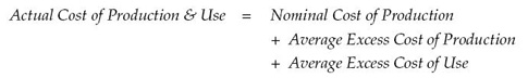
Let us define the effective cost of production and use as:
The actual cost of producing and using an item (the numerator) will consist of the nominal cost of production plus the average excess costs per unit associated with producing and using such items.
Thus, to determine the effective cost of production and use, we will need to characterize these average excess costs. These excess costs can be broken down into three components: the costs of scrap, the costs of rework, and the excess costs associated with the use of conforming product. To create our excess cost function, we shall need to look at each of these three excess costs.
Defining an excess cost function
Because scrapping an item is a cut-your-losses action—ideally taken only when it is cheaper to scrap the item than to use it—we can think of the cost of scrap as a fixed cost. That is, let CS denote the cost of scrapping an item. This cost will have to equal the cost of the raw materials plus the cost of all processing done to the item, the cost of inspection, and perhaps the cost of disposal as well. In figure 1, this fixed cost of scrapping an item is denoted by a horizontal line beyond the lower specification limit, LSL.
Let CR denote the average cost of reworking an item. This cost will usually be less than or equal to the cost of scrapping the item. In figure 1 this average cost of reworking an item is denoted by a horizontal line beyond the upper specification limit, USL.
Thus, we know the excess cost function in two regions—scrap and rework. To fill in the rest of the curve, we need to think about the nature of excess costs. Excess costs are the result of variation. They are costs incurred because everything is not right at the target value. If we could make everything right at the target value, there would, by definition, be no excess costs of production. Therefore, we define the excess costs to be zero at the target value, and this gives us a third point for the excess cost function, as shown in figure 2.
But how do we fill in the gaps? Because we know that small deviations from the target can be tolerated, we prefer to use quadratic curves to connect the three known portions of the excess cost function. These quadratic curves will have their minimum at the target value, and will connect with the fixed portions of the excess cost function to give the piecewise continuous curve shown as L(x) in figure 3.
This excess cost function suggests that when an item falls near the target, there will be few excess costs associated with its use. However, as an item falls further and further away from the target, the costs of using the item will increase. Moreover, these costs will increase up to that point where it will be cheaper to scrap or rework the item than it will be to try to use it. Because this is consistent with reality, the curve in figure 3 is a realistic excess cost function.
It is important to note that the excess cost function in figure 3 is completely determined by the three points shown as black dots. (Because each quadratic curve has a vertex at the target value, each quadratic curve is fully defined by the target value and one of the other two points.) It is this property of our realistic excess cost function that will allow us to use the capability and performance indexes to obtain the excess costs.
Average excess costs
In figure 3, the probability model f(x) represents the product distribution. Whether it is a description of the past or a prediction for the future does not matter at this point. When we multiply the excess cost function L(x) by the probability model f(x) and then integrate over all values of x, we end up with the weighted average excess cost of production and use.
The portion of this integral where x is between the specifications will define the average excess costs of use. The two portions of this integral where x is outside the specifications will define the average excess costs of production. Thus, we have in this one integral the last two parts of the numerator defined earlier:
Returning to the definition of the effective cost of production and use, we have:
where the last two quantities are expressed as a percentage of the nominal cost. Thus, the effective cost of production and use is a multiplicative value that expresses the amount by which the actual costs of production and use exceed the nominal cost of production. It can be used in this form, or it can be converted into dollars by multiplying by the nominal cost of production.
Where do the capabilities come in?
The three points that define the excess cost function in figure 3 occur at the target and the specifications. The relationship between the process outcomes and the specifications is characterized by the capability indexes. Thus, for a given situation, it is possible to express the excess cost of production and the excess cost of use as a function of the capability indexes. Tables based on this relationship will allow you to convert the capability indexes directly into excess costs of production and excess costs of use without having to actually evaluate the integral defined above. To illustrate this we shall use as an example the baseline computation for the Tokai Rika Cigar Lighter detent dimension. In what follows I will compare the direct computation of the effective cost of production and use with the table look-up approach.
Figure 4 gives the data for the Tokai Rika Lighter Detent Dimension. Four pieces are measured each day and arranged into daily subgroups. The first 24 days of production are used as the baseline period for computing the limits for the Average and Range Chart shown in figure 5. The values recorded are in hundredths of a millimeter in excess of 15.00 mm. Thus, the target value of 15.90 mm is shown as 90. The specifications are 80 to 100. The grand average is 89.80 and the average range is 3.04. When the average range is divided by the bias correction factor for subgroups of size four we end up with a value for Sigma(X) of 1.48. Assuming that nonconforming items are scrapped we end up with a symmetric excess cost function like that in figure 6.
The capability indexes for these data are:
Using a table for the situation where all nonconforming product is scrapped, and rounding these capability indexes off to 2.30 and 2.20, we can convert these capability indexes into the following excess costs:
For this process Tokai Rika has excess costs that amount to about 2 percent of the nominal costs. All of these excess costs are excess costs of use, which is consistent with figure 6. To see how these excess costs were obtained, consider the following direct evaluation approach.
The natural process limits for this process are 85.4 to 94.2. These values fall well within the specifications of 80 to 100, as shown in figure 6. Because we will only need to evaluate the integral over this reduced range of values, our generalized excess cost function of figure 3 effectively becomes a simple quadratic equation of the form:
Whenever the excess cost function is a quadratic equation, the average excess cost will always reduce down to the following expression regardless of which probability model f(x) is used:
where µ is the mean of f(x), σ is the standard deviation of f(x), and K is a constant that defines the quadratic curve and converts everything into monetary units. Inspection of this perfectly general result will show that the average excess cost will always be minimized by operating on target with minimum variance.
We may evaluate the expression for the average excess cost using:
If we assume that the cost of scrapping a lighter shell is the same as the nominal cost of production, and that this cost, in Yen, is CS = ¥ 20, then we have:
Thus, the effective cost of production and use for this process is estimated to be:
Whether by direct computation, or by simply converting the capability indexes, we arrive at the effective cost of production and use for this process. Tables for converting capability indexes into (1) the excess cost of production, (2) the excess cost of use, and (3) the effective cost of production and use may be found in my new book, Reducing Production Costs (SPC Press, 2010). How you can use the effective cost of production and use to define entitlements and potential returns for improvement projects will be the topic of my September column.
Comments
Convincing Management To Take Action
How does one convince an operations manager that loss is occuring and action should be taken to center the process when the Cp and Cpk are greater than 2? Especially, with no defects occurring, how do you convince the manager that loss is occurring?
Ignorance Is Bliss
Ignorance is indeed bliss. The production manager needs educating, not convincing. He/she can only convince themselves.
Add new comment