Our PROMISE: Our ads will never cover up content.
Our children thank you.
Donald J. Wheeler
Published: Tuesday, May 31, 2011 - 11:03 Whenever we present capability indexes the almost inevitable follow-up question is, “What is the fraction nonconforming?” What this question usually means is, “Tell me what these capability indexes mean in terms that I can understand.” These questions have resulted in multiple approaches to converting capability indexes and performance indexes into fractions nonconforming. This article will review some of these approaches and to show their assumptions, strengths, and weaknesses. In order to make the following discussion concrete, we will need an example. We shall use a collection of 100 observations obtained from a predictable process. These values are the lengths of pieces of wire with a spade connector on each end. These wires are used to connect the horn button on a steering wheel assembly. The upper specification for this length is 113 mm. The oldest and simplest approach to estimating the fraction nonconforming is arguably the best approach. Here the estimate of the fraction nonconforming is simply the number of observed values that are outside the specifications, Y, divided by the total number of observed values, n. The name commonly used for this ratio is the “binomial point estimate”: This ratio provides an unbiased estimate of the process fraction nonconforming. For the data of figure 1, the specifications are 97 mm to 113 mm. Six of the observed values exceed 113, so Y = 6, n = 100, and our binomial point estimate for the fraction nonconforming is p = 0.06 or 6 percent. Note that the reference to the binomial distribution does not apply to the wire lengths, X, but rather to the counts Y and n. This approach makes no assumptions regarding the histogram in figure 1. No probability model is assumed. No lack-of-fit tests are used. Just count how many values are outside the specifications and divide by the total number of observed values. If the data come from 100-percent inspection, then there is no uncertainty in the descriptive ratio above. The 6 percent is the fraction rejected at inspection, and the only uncertainty is the uncertainty of misclassification, as described in my column last month. However, if we are using the data of figure 1 for representation or prediction, then we will have to be concerned with the uncertainty involved in the extrapolation from the product measured to the product not measured. In this case the production process was being operated predictably, so this extrapolation makes sense. (To read more about representation and prediction see my April column, “How Measurement Error Affects the Four Ways We Use Data.”) When data are used for representation or prediction, we will need to use an interval estimate in addition to the point estimate. The interval estimate will define the range of values for the process fraction nonconforming that are consistent with the observed point estimate. Most textbooks will give a formula for an approximate 95-percent interval estimate that is centered on the binomial point estimate p: This formula was first given by French mathematician Pierre Simon Laplace in 1812 and is today commonly referred to as the “Wald interval estimate.” Although this simple approximation is satisfactory when the proportions are in the middle of the range between 0.00 and 1.00, it does not work well for proportions that are close to either 0.00 or 1.00. Since the fraction nonconforming will hopefully be near 0.00, we will need to use a more robust interval estimate given by E. B. Wilson in 1927. The 95-percent Wilson interval estimate will be centered on a value known as the “Wilson point estimate”: This Wilson point estimate effectively shifts the center of the interval estimate so that the formula will yield a more appropriate interval. Using Y = 6 and n = 100, the Wilson point estimate is 0.0769, and the 95-percent Wilson interval estimate for the process fraction nonconforming is: So using the specifications above, the data in figure 1 give us a binomial point estimate of 6 percent, and a 95-percent Wilson interval estimate for the process fraction nonconforming of 2.6 percent to 12.8 percent. While 6 percent nonconforming is our best point estimate, the uncertainty of the extrapolation from our observed values to the underlying process means that our observed value of 6 percent nonconforming is consistent with a process that is producing anywhere from 2.6 percent to 12.8 percent nonconforming. If we changed the upper specification to be 114 mm, then Y would be 3, the binomial point estimate would be 3 percent, and the 95-percent Wilson interval estimate would be 0.0481 ± 0.0411. Thus, an observed value of 3 percent nonconforming would be consistent with a process fraction nonconforming of 0.7 percent to 8.9 percent. Now consider what would happen if the upper specification was 116 mm. Here Y would be 0, the binomial point estimate would be 0 percent, and yet the 95-percent Wilson interval estimate would be 0.0192 ± 0.0264. Thus, our observed value of 0.0 percent nonconforming would be consistent with a process fraction nonconforming of 0.0 percent to 4.6 percent. Since Y can not get any smaller than zero, this last interval estimate reflects the limitations of the inferences that can be drawn from 100 observed values. Processes producing less than 4.6 percent nonconforming can, and will, produce some 100 piece samples that have zero nonconforming items! Thus, the Wilson interval estimate provides us with a way to characterize the process fraction nonconforming based on the observed fraction nonconforming. It defines the uncertainty that is inherent in any use of the data to estimate the process fraction nonconforming. Sometimes, rather than using the data to directly estimate the fraction nonconforming, a probability model is fitted to the histogram and used to compute the tail areas beyond the specification limits. While the data are used in fitting the probability model to the histogram, the estimate of the fraction nonconforming will be obtained from the fitted model rather than the data. As an example of this approach we will fit a normal distribution to the wire length data from figure 1. The wire length data have an average of 109.19 mm, a standard deviation statistic of 2.82 mm, and the process behavior chart shows no evidence of unpredictable operation while these values were obtained. A normal probability model having a mean of 109.19 and a standard deviation parameter of 2.82 is shown superimposed on the histogram in figure 2. As before, we begin with the assumption that the upper specification limit is 113 mm. In the continuum used by the model, this becomes 113.5 mm. When we standardize 113.5 mm, we obtain a z-score of 1.53, and from our standard normal table we find that this corresponds to an upper tail area of 0.0630. Thus, using a normal probability model we obtain a point estimate of the process fraction nonconforming of 6.3 percent, which is not much different from the empirical estimate found earlier. So, just how much uncertainty is attached to this estimate? Judging from the few cases where the formulas for interval estimates are known, we can say that if the probability model is appropriate, then this estimate is likely to have a slightly smaller interval estimate than the empirical approach. However, if the probability model is not appropriate, then this estimate can have substantially more uncertainty than the empirical estimate. Which brings us to the first problem with this approach: Any choice of a probability model will, in the end, turn out to be an unverifiable assumption. It amounts to nothing more than an assertion made by the investigator. While lack-of-fit tests may sometimes allow us to rule out a probability model, no test will ever allow us to validate a particular probability model. Moreover, given a sufficient amount of data, you will always detect a lack of fit between your data and any probability model you may choose. This inability to validate a model is the reason that it is traditional to use the normal distribution when converting capabilities into fractions nonconforming. Since the normal distribution is a maximum entropy distribution, its use amounts to performing a generic, worst-case analysis. (It is important to note that this use of a normal distribution is a matter of convenience, arising out of a lack of information, and is not the same as an a priori requirement that the data “be normally distributed.”) To illustrate the generic nature of estimates based on the normal distribution, we will use the ball-joint socket thickness data shown in figure 3. There we have 96 values collected over the course of one week while the process was operated predictably. The average is 4.667, and the estimated standard deviation is 1.80. The first probability model fitted to these data is a normal distribution having a mean of 4.667 and a standard deviation parameter of 1.80. There is a detectable lack of fit between the histogram and this normal distribution. The second probability model fitted to these data is a Burr distribution with c = 1.55 and k = 58.55 that has been shifted to have a mean of 4.667 and stretched to have a standard deviation parameter of 1.80. There is no detectable lack of fit between this Burr distribution and the histogram. When working with skewed histograms like the one in figure 3, we are primarily concerned with areas in the long tail because the short tail is usually restricted by a barrier or boundary condition. Considering the discrete values found in these data we will consider the upper tail areas defined by the cutoff values of 5.5, 6.5, 7.5, etc. The table in figure 4 shows these upper tail areas computed three ways: (1) using the normal distribution, (2) using the fitted Burr distribution, and (3) using the empirical binomial point estimate. Finally, the last two columns in figure 4 give the lower and upper bounds for the process fraction nonconforming based on the 95-percent Wilson interval estimates. As expected, the estimates based on the normal probability model differ from those found using the Burr probability model. Moreover, these estimates also differ from the binomial point estimates shown in the third column. However, in each row, all three estimates fall within the bounds defined by the 95-percent Wilson interval estimate. This illustrates what will usually be the case: The uncertainty inherent in the data will usually be greater than the differences between the various estimates. This makes any discussion about which estimate is best into a mere argument about noise. When we are estimating the fraction nonconforming, the uncertainty in our estimates will generally overwhelm the differences due to our choice of probability model. The numbers you obtain from a probability model are not really as precise as they look. And that is why the generic ballpark values obtained by using a normal distribution will usually be sufficient. (Remember, the normal distribution displayed a detectable lack of fit for these data, and yet all of the normal estimates fell within the intervals defined by the uncertainty in the empirical estimates.) “But using a fitted probability model will let us compute tail areas for capability indexes greater than 1.00,” you say. Yes, it will, and that is the second problem with the probability model approach. No matter how many data you have, there will always be a discrepancy between the extreme tails of your probability model and the tails of your histogram. This happens simply because histograms always have finite tails while probability models usually have at least one infinite tail. The table in figure 5 shows the average size of the finite tails of a histogram. There I have listed the average distances between the average of a histogram and the maximum value for that histogram. These distances are given in standard deviation units. Once you get beyond 200 data, the tails of the histogram grow ever more slowly with increasing amounts of data. While most of the values in figure 5 have been known since 1925, this aspect of data analysis has seldom been taught to students. These values show that the major discrepancies between a probability model and a histogram are generally going to occur in the region out beyond three standard deviations on either side of the mean. Call this region the extreme tails of the probability model. When we are converting capability indexes that are less than 1.00 into a fraction nonconforming, these discrepancies in the extreme tails between our histogram and our probability model will not have much of an impact. (Six percent nonconforming plus or minus 60 parts per million is still 6 percent nonconforming.) But, when your capability indexes get to be larger than 1.00, any conversion will require the computation of infinitesimal areas under the extreme tails of the assumed probability model. Here small differences in the probability model can result in dramatic changes in the computed values. (Sixty parts per million plus 60 parts per million will be 120 parts per million.) To illustrate this, figure 6 will extend the table of figure 4 to cutoff values beyond three sigma. Here the upper tail areas are given in parts per million: The upper specification limit for the socket thickness data is 15.5. Which estimate from figure 6 should you tell your boss? 1 ppb? 24 ppm? Or something less than 4.7 percent? When we get beyond three sigma we find considerable differences between the upper tail areas of the two different probability models. At the upper specification cutoff of 15.5, these areas differ by a factor of 24,000. However, all 18 estimates in figure 6 are estimates of a process fraction nonconforming that, according to the data, falls somewhere between 0 percent and 4.7 percent. While our assumed probability models allow us to compute numbers out to parts per million and parts per billion, the data themselves will not support an estimate that is more precise than to the nearest five parts per hundred. Think about this very carefully. When you compute tail areas out beyond three sigma, you are computing values that are entirely dependent upon the assumed probability model. These tail areas will have virtually no connection to the original data. Because of the inherent discrepancy between the tails of the histogram and the tails of the probability model, converting capability indexes that are larger than 1.00 into fractions nonconforming will tell you more about the assumed model than it will tell you about either the data or the underlying process. This is why such conversions are complete nonsense. Thus, there are two problems with using a probability model to estimate the process fraction nonconforming. The first is that any choice of a probability model is essentially arbitrary, and the second is that the use of a probability model encourages you to extrapolate beyond the tails of the histogram to compute imaginary quantities. Given the uncertainty attached to any estimate of the process fraction nonconforming, the choice of a probability model will usually make no real difference as long as the capability indexes are less than 1.00. Here the use of a generic normal distribution will provide reasonable ballpark values, and there is little reason to use any other probability model. However, when the specifications fall beyond the tails of the histogram, and especially when the capability indexes exceed 1.10, no probability model will provide credible estimates of the process fraction nonconforming. Computing an infinitesimal area under the extreme tails of an assumed probability model is an exercise that simply has no contact with reality. The histogram shows us what we know, and it also reveals what we do not know. When we add an assumed probability model to our histogram we are adding ink that does not represent the data. The technical term for such nondata-ink is “chartjunk.” Like a stage magician’s props, this chartjunk serves to distract our attention from the reality of the histogram and to usher us into the realm of illusion and make-believe. What we know depends upon how many data we have and whether or not those values were collected while the process was operated predictably. Moreover, the only way to determine if the data were obtained while the process was operated predictably is by using a process behavior chart with rational sampling and rational subgrouping. If the data show evidence that the process was changing while the data were collected, then the process fraction nonconforming may well have also changed, making any attempt at estimation moot. (In the absence of a reasonable degree of predictability, all estimation is futile.) If the data show no evidence of unpredictable operation, then we may use the binomial point estimate to characterize the process fraction nonconforming. In addition we may also use the 95-percent Wilson interval estimate to characterize the uncertainty in our point estimate. This approach is quick, easy, robust, and assumption free. When no observed values fall beyond a specification limit, our count Y becomes zero and the binomial point estimate goes to zero. However, the 95-percent Wilson interval estimate will still provide an upper bound on the process fraction nonconforming. These upper bounds will depend solely upon the number of observations in the histogram, n. Selected values are shown in the table in figure 8. The upper bounds listed in figure 8 define the essential uncertainty in all estimates of the fraction nonconforming that correspond to Y = 0. This means that when you use a probability model to compute a tail area that is beyond the maximum or the minimum of your histogram, then regardless of the size of your computed tail area, the process fraction nonconforming can be anything up to the upper bound listed in figure 8. There we see that it takes more than 1,000 data to get beyond the parts-per-hundred level of uncertainty. Say, for example, that you have a histogram of 70 data collected while the process was operated predictably and on-target with an estimated capability ratio of 1.33. Say that these data are suitably bell-shaped and that you use a normal distribution to estimate the process fraction nonconforming to be 64 parts per million. Figure 8 tells us that with only 70 data, all you really know about the process fraction nonconforming is that it is probably less than 6.4 percent nonconforming. This is 1,000 times the computed value of 64 ppm! With this amount of uncertainty, how dogmatic should you be in asserting that the process fraction nonconforming is 64 parts per million? Until you have hundreds of thousands of data collected while the process is operated predictably, you simply do not have any basis for claiming that you can estimate the fraction nonconforming to the parts-per-million level. One day a client from a telephone company observed that they computed the number of dropped calls each day in parts per million. However, in this case they were using the empirical approach and the denominator was in the tens of millions. With this amount of data the uncertainty in the computed ratio was less than 0.5 ppm, and reporting this number to the parts-per-million level was appropriate. But for the rest of you, those who have been using a few dozen data, or even a few hundred data, as the basis for computing parts-per-million nonconforming levels, I have to tell you that the numbers you have been using are no more substantial than a mirage. The uncertainties in such numbers are hundreds or thousands of times larger than the numbers themselves. The first lesson in statistics is that all statistics vary. Until you understand this variation, you will not know the limitations of your computed values. Using parts per million numbers based on a few hundred data without regard to their uncertainties is a violation of this first lesson of statistics and is a sign of a lack of understanding regarding statistical computations. Quality Digest does not charge readers for its content. We believe that industry news is important for you to do your job, and Quality Digest supports businesses of all types. However, someone has to pay for this content. And that’s where advertising comes in. Most people consider ads a nuisance, but they do serve a useful function besides allowing media companies to stay afloat. They keep you aware of new products and services relevant to your industry. All ads in Quality Digest apply directly to products and services that most of our readers need. You won’t see automobile or health supplement ads. So please consider turning off your ad blocker for our site. Thanks, Dr. Wheeler is a fellow of both the American Statistical Association and the American Society for Quality who has taught more than 1,000 seminars in 17 countries on six continents. He welcomes your questions; you can contact him at djwheeler@spcpress.com. Estimating the Fraction Nonconforming
How to know what the data are really telling you
The empirical approach
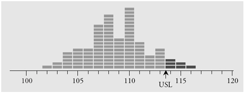
Figure 1: Histogram of 100 wire lengthsThe probability model approach
Figure 2: A normal distribution fitted to the wire length data
Figure 3: Two probability models fitted to the socket thickness data
Figure 4: Three different estimates of upper tail areas
Figure 5: Histogram tails grow very slowly with increasing n
Figure 6: Estimating extreme upper tail areas
Figure 7: The difference between chartjunk and data So what do we really know?
Figure 8: The uncertainty in estimates of fractions nonconforming when Y = 0
Our PROMISE: Quality Digest only displays static ads that never overlay or cover up content. They never get in your way. They are there for you to read, or not.
Quality Digest Discuss
About The Author
Donald J. Wheeler
© 2023 Quality Digest. Copyright on content held by Quality Digest or by individual authors. Contact Quality Digest for reprint information.
“Quality Digest" is a trademark owned by Quality Circle Institute, Inc.
Comments
Lazy and Uneducated?
I think I'll stick with the binominal point estamate. Easy to explain, simple to calculate and relies on no assumptions. But then again...perhaps I'm one of those uneducated and lazy folks (NOT).
THERE ARE PEOPLE WHO ARE AFRAID OF CLARITY BECAUSE THEY FEAR THAT IT MAY NOT SEEM PROFOUND.
Elton Trueblood.
Rich DeRoeck
Fraction Nonconforming
Elton and Rich:
For the sake of clarity, I recommend you read: "Statistics Without Tears", or, "The Idiot's Guide to Statistics", or, "Statistics for the Utterly Confused" so in the future, you can simplify your world of statistics. These books can be found at Amazon.com. Profound, these books are NOT, but such clarity and so simple to use, you'll feel like you're back in junior high math class. Enjoy.
David A. Herrera
Estimating the Fraction Nonconforming
Dr. Wheeler should have stated his case for individuals control charts, because this is where many prominent world renowned quality and industrial engineers and statisticians disagree with him in the PHASE II of SPC monitoring. I agree that fitting a normal distribution to everything may not matter much when a process is unstable for several reasons. Any assignable cause will be investigated and the SPC chart will be rerun after the cause is found and the part fixed. Individuals control charts are very sensitive to non-normality. Type II (false alarm) errors occur when fitting a normal distribution to skewed data. A normal distribution is NOT "good enough" when fitting skewed, non-normal data to create an SPC chart. Control limits should be computed from the best-fitted distribution when the data is significantly skewed, not from a normal distribution. Dr. Wheeler infers all probability plots are useless, because he says everyone should fit a normal distribution to all data.
As for fraction-nonconforming, NO ONE chooses a probability model randomly or arbitrarily. Statisticians and Systems Engineers choose the BEST distribution based on a GOODNESS OF FIT statistic, such as the Anderson-Darling statistic, the Kolmogorov-Smirnov statistic, or others. Dr. Wheeler slams Goodness of Fit statistical theories, which have been useful proven tools in modeling and simulations, because these models and simulations are tested over and over and verified. Dr. Wheeler goes against past and present eminent scientists and engineers who use Goodness of Fits and use probability plots every day in their work. Dr. Wheeler also goes against hypothesis testing and using probability plots to weed out bad fits in order to compute fraction nonconforming more accurately.
All probability distributions can be tested for Goodness of Fits to properly model the data; if the normal is the best fitting one, so be it. If not, a non-normal distribution should be used to compute the Probability of Nonconformance (PNC); this is the fraction non-conforming in percent. Assuming a two-sided limit, the Yield = 100% - (total PNC of upper and lower spec limits). Dr. Wheeler failed to note that a best-fitted probability distribution can also have 95% confidence limits, so why compare a badly fitting normal distribution to skewed data and claim it's appropriate? It is not appropriate.
Six-sigma is a process that uses sound and robust statistics to ensure a wider margin of quality for acceptance testing, ensuring zero rework, and shipping products to customers with no returns or flaws. Several companies have saved millions of dollars using a well-planned and implemented six sigma process. What sticks out more than anything else about Dr. Wheeler's comments on fraction non-conforming are the risks in REWORK caused by his assumption of normality in SPC charts and using the Poisson or binomial distribution to compute fraction non-conforming for all cases (using the empirical method). Using the binomial distribution or empirical method of X successes out of N samples is merely using the old bean-counting PASS/FAIL system of the last century: this method gives no information about the probability of rework like a well-fitted probability model does. Also, regarding using 95% confidence limits, is 5% error margin good enough to send products with this fraction nonconforming error margin to the customer? Do aerospace companies want to live with 5% probability of rework???
In summary I think Dr. Wheeler is going against too many well established probability and statistical methods and many statistical and industrial engineering experts by oversimplifying fraction nonconformance to the point of causing rework if companies were to adopt Dr. Wheeler's approach. Rework of course can be translated into dollars as Dr. Genichi Taguchi pointed out. Caution is advised in oversimplifying models thinking they are "good enough" to fit the real world and good enough to avoid rework.
One last note: Businesses and engineering methods and quality suffer due to lazy and uneducated people who hate to do statistics. Six-sigma haters have a point in hating six sigma only when their six sigma program is run by charlatans who do NOT use probability and statistics at all or misuse it. These people should know that common sense mixed with 21st Century engineering and technology, and education in mathematics, gets PROVEN results while others can only speculate and get rework from their SPC programs.
"statistics haters" and other lazy people
David - I'm not disputing that we can often find an appropriate distributional model to predict the fraction nonconforming - often we can. But I think you may have missed Dr. Wheeler's point, which is that many people have leraned the 'dumbed down' version of statistics and many people in industry use them. The situation that Dr. Wheeler describes (the rote appliation of the Normal distribution to predict defect rates when none are are observed becuase the process is stable well withinthe limits) is an epidemic in industry. This epidemic applies not only to the frequency but the severity of its mis-use. You are correct that such people are ignorant - and/or lazy - but yet they continue on in their blissfully ignorant way much like the mayhem guy on the insurance commercials. We need to get thru to them - not you or your organization. Although this behavior is no longer tolerated within my organization, I am continually retraining new hires (fresh out of university and with 35 years of experience) and my suppliers.
Another comment I would make is that although we can determine a suitable distribution, we often don't need to. Will a more sophisticated calculation change the action we need to take? a 5% defect rate calculated simply from the observed defect rate will not drive a different action than using a probability distribution to predict the likely rate to be 5.16% On the other hand I do use fairly sophisticated models on board diagnostic equipment to ensure that even a small percentage of bad runs don't occur...it all depends.
Education
Thanks for the common sense. I have several thousand users of a software that reports estimated nonconforming fractions. Most of them treat those ppm's as if they were the "real" thing. I've been looking for a way to explain the uncertainity associated with those estimations. May I cite your article Dr. Wheeler? or maybe Mr. Wilson's work?
Another Eye-opening article!
Great new insight, as usual, Don. I've been doing some work to try to get rid of the "Process Sigma Table" used almost universally in the Six Sigma world. This is just more ammunition.
More uncertainty
This article is excellent. I didn't realize there is so much uncertainty surrounding these summary statistics. And to think this doesn't even account for sampling and inspection errors.
Rich DeRoeck
Estimating Fraction noncomforming
I am not a statistician but am trying desperately to learn the ropes; I understood this article well until we got to The Probability Approach and Z values; I know about normal distribution, the Standard Normal Table and all but for a novice like myself this article misses the mark. Many times I run into the same problem, that is that knowledgable authors begin by explaining in basic terms and concepts and then as the article goes on they forget their audience (I only assume the novice is your audience) and become too technical and lose me; the novice. Where can I get the Real Dummies guide to these topics where complex ideas are broken down into simple application
Sorry About the Confusion.
The latter half of this article was focused on a practice that is widely used and seriously misunderstood. If you can use the first part then that is all that you need to avoid serious confusion. The Binomial Point Estimate is vary easy to compute, and the Wilson Interval Estimate is not much harder. The use of probability models, z-scores, and all that is something that you really do not need in practice. So, hopefully this will relieve some of the anxiety.
No Dummies Guide
I don't know that there is a good "Dummies" guide to any of this...Marilyn Vos Savant demonstrated years ago that many Ph.D. mathematicians are dummies when it comes to probabilities (Google "Monty Hall Dilemma" if you want more info on that). The problem is that probability concepts are counterintuitive for most people. Add to that that most stats teachers and authors only approach stats from three of its inherent problems: probability models, descriptive statistics, and inferential statistics. They give very little, if any, attention to the fourth problem--homogeneity.
If you know the standard normal tables, then you know what Z values are (standard deviation distances from zero in the standard normal distribution). A great guide to some of the concepts in this article is Don Wheeler's "Making Sense of Data." It's pretty accessible. Davis Balestracci's Data Sanity is very helpful, as well.
Six Sigma
Hopefully this article starts to get through the thick heads of the thousands of companies who have been conned into paying billions of dollars on ridiculous six sigma programs.
Hopefully one day Six Sigma will be sent to history's trash can of global follies. Will there ever be a return to clear thinking ?
Practical vs. Theoretical
Thanks again for bridging the gap between the theoretical (i.e., Six Sigma thinking) and the real world. Although he may not like the answer, I would far rather tell my boss our defect rate was less than say, 6.4% (based on real data) than give him some number like 3.4 ppm!!!