Problems With Skewness and Kurtosis,
Part 2

What do the shape statistics do?

Published: Monday, August 1, 2011 - 15:11

In part one we found that the skewness and kurtosis parameters characterize the tails of a probability model rather than the central portion, and that because of this, probability models with the same shape parameters will only be similar in overall shape, not identical. However, since software packages can only provide shape statistics rather than shape parameters, we need to look at the usefulness of the shape statistics.

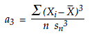
In part one, we saw that the skewness parameter is the third standardized central moment for the probability model. For this reason, a commonly used statistic for skewness is the third standardized central moment of the data:

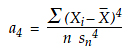
In a similar manner, we shall use the fourth standardized central moment of the data as our statistic for kurtosis:

Since both of the formulas above use the root mean squared deviation, s_n, rather than the more common standard deviation statistic, s, there may be slight differences between the statistics listed above and the statistics given by your software. For example, Microsoft Excel uses the formulas:

Regardless of the different formulas, a₃ contains the essence of all statistics for skewness while a₄ contains the essence of all statistics for kurtosis. For this reason we shall use the simple a₃ and a₄ statistics here.

To illustrate these shape statistics, I shall use the 200 observations shown in figure 1. These represent the values logged during a 20-day period of production. The descriptive statistics for these 200 values are: The average is 256.46; the standard deviation statistic is 4.58; the skewness ( a₃ ) is 1.60; and the kurtosis ( a₄ ) is 6.31. (The Excel formulas result in values of 1.61 and 3.42, respectively.) The histogram for these values is shown in figure 2. This histogram looks like many histograms that come from process related data. The bulk of the values fall in a central mound while some of the values trail off to one side in an elongated tail.

Figure 1: Values from 20 days of production

Figure 2: Histogram for the 200 data of figure 1

Although the descriptive statistics do correctly characterize the data shown in the histogram in figure 2, this is not the same as using these descriptive statistics to estimate the parameters of a probability model. Whenever we use statistics to estimate parameters we will need to take into account the inherent uncertainty attached to our estimates.

When we use the average to estimate the mean of a probability model, the uncertainty is a function of the inverse of the square root of n. That is, the standard deviation of the average statistic is given by:

where σ is the standard deviation parameter of the probability model and n is the number of values used to compute the average.

Next consider using the standard deviation statistic to estimate the standard deviation parameter of a probability model. Here the uncertainty will be a function of the inverse of the square root of twice the number of data. Specifically, the standard deviation of the standard deviation statistic will be:

This value will be about 71 percent as large as the uncertainty in the estimate of the mean parameter.

Thus, with any given data set, we will always estimate the location and dispersion parameters with about the same amount of uncertainty.

When we use a skewness statistic to estimate the skewness of a probability model, the uncertainty will be 2.45 times the uncertainty in the estimate of the location parameter since:

When we use a kurtosis statistic to estimate the kurtosis of a probability model, the uncertainty will be about 4.9 times the uncertainty in the estimate of the location parameter since:

These four results mean that we will always estimate the location and dispersion with greater precision than we will ever estimate the shape parameters. For example, if we use 20 data to estimate the mean, and if we then wanted to also estimate the skewness with a similar precision, we would need to collect and use 120 data to estimate the skewness. Likewise, it would take 480 data to estimate the kurtosis with the same precision that we can achieve when using 20 data to estimate the mean.

This means that regardless of how many data we have, we will always have much more uncertainty in the shape statistics than we will have in the location and dispersion statistics.

This limitation on what we can obtain from a collection of data is inherent in the statistics themselves, and must be respected in our analysis of the data.

Using the formulas above, we will compute approximate 95-percent interval estimates for the mean, standard deviation, skewness, and kurtosis of the process that produced the data in figure 2.

These approximate 95-percent interval estimates will have the form:

So, with our 200 data, we would estimate the process mean to be about 256.5 plus or minus 0.6. We would estimate the process standard deviation to be about 4.6 ±0.5. Our skewness could be anywhere from 0.0 to 3.2, and our kurtosis could be anywhere between 3.1 and 9.5!

Figure 3: The inherent uncertainties in shape statistics

Figure 4: The region likely to contain a model for the process of figure 2

Since the shape characterization plane uses the square of the skewness on the horizontal axis, the 95-percent interval estimates above refer to points within the red rectangle shown in figure 4. This rectangle essentially covers the heart of the shape characterization plane.

Based on the uncertainty in our statistics for skewness and kurtosis we can rule out the platykurtic probability models and possibly the normal distribution as well, but very little else.

Thus, with 200 data, our estimates of skewness and kurtosis are simply not sufficient to identify a particular probability model, or even a reasonably small group of probability models, to use in characterizing this production process.

Thus, the first problem with the shape statistics of skewness and kurtosis is simply this: Until thousands of data are involved in the computation, the shape statistics will have so much uncertainty that they will not provide any useful information about which probability models might be reasonable candidates for a process. Any attempt to use the shape parameters to identify which probability model to use will always require more data than you can afford to collect. But even if you could afford enough data, there are two more problems that create a barrier to using the shape statistics.

The second problem is that the shape statistics depend upon the extreme values of the histogram. As we saw in part one, the shape parameters characterize the tails of a probability model. In a similar manner, the shape statistics will be more dependent upon the extreme values in the data than they will on the data set as a whole.

To illustrate this, figure 5 shows the cumulative values for the shape statistics for figure 2. Here we see how the values for the skewness and kurtosis statistics change as additional data are used in the computation. The first row shows the shape statistics based on days 1 through 5 (50 data). The second row shows these values based on days 1 through 10 (100 data). Row three uses days 1 through 15. Row four uses days 1 to 17. Row five uses days 1 to 19. Row six uses all 20 days. There we see that these statistics do not converge to fixed values as the amount of data increases.

Figure 5: The shape statistics for figure 2 do not converge with increasing amounts of data

Figure 6 shows the points of figure 5 plotted in the shape characterization plane. We would expect this graph to show a series of points that get closer together, with the distance between successive points getting smaller as the amount of data increases. This is what will happen when a statistic converges to the value of some process parameter. However, in figure 6 we see the sensitivity to extreme values that is inherent in all shape statistics. Here the jump from the point for n = 190 to the point for n = 200 is larger than all of the preceding line segments put together. Ten data points out of 200 amount to only 5 percent of the data, yet they move the point in figure 6 from (0.36, 3.21) to (2.54, 6.31). This is a strong indication that the process represented by the data of figure 2 is changing. And when the process is changing, the notion of process parameters is not well-defined. This leads to the third problem with the use of the shape statistics.

Figure 6: The random walk of the shape statistics for figure 2

This third problem has to do with the implicit assumptions behind the descriptive statistics. As the name implies, these statistics describe various aspects of the data set for which they were computed. That is, they will characterize the data. Whether these statistics can be used to estimate a process parameter is a much more complex question. Before we can use a statistic to estimate a parameter, we will have to have a set of data for which it makes sense to talk about a probability model. And the primary requirement for a probability model to make sense is that the data are homogeneous.

This means that whenever we use a descriptive statistic to estimate a process characteristic, we are making a very strong assumption that the data are homogeneous.

Thus, while we may always compute our descriptive statistics, we cannot begin to use those statistics to estimate process parameters until we know that the data set is homogeneous. And the only completely general technique that can examine suspect data for evidence of a lack of homogeneity is the process behavior chart.

Figure 7 shows the average and range chart for the data of figure 2. There I used the data from each day as a subgroup, resulting in 20 subgroups of size 10. The limits were computed using all of the data. The grand average is 256.46, and the average range is 5.90. Thirteen of the 20 subgroup averages fall outside their limits, which means that this process was operated differently at different times. The first six days seem to show a process that was operated at one level. The next six days show a process that was operated at a slightly higher level. The last eight days show a process that has gone on walkabout. Thus, the data of figure 2 are definitely not homogeneous. The histogram in figure 2 does not represent any one process, but instead it represents an unknown mixture of several different processes.

Figure 7: Average and range chart for the data of figure 1

When the data are not homogeneous, our descriptive statistics become misleading. While the statistics describe the data, the data are a meaningless blend of values obtained under different conditions. In figure 7 we used the grand average of 256.5 as the central line for the average chart, yet this chart shows that the process average was detectably different from 256.5 on 13 of the 20 days.

The descriptive standard deviation statistic of 4.58 units is more than twice the size of the more robust estimate of 1.92 units obtained from the average range.

The skewness statistic of 1.60 is simultaneously inflated by the random walk of the process and simultaneously deflated by the excessively large value for the standard deviation statistic. In figure 4 we saw that there is so much uncertainty in this statistic that it does not begin to narrow the possibilities. This statistic simply contains no useful information.

The kurtosis statistic of 6.31 was heavily inflated by the last subgroup. It was also simultaneously deflated by the excessively large value for the standard deviation statistic. In figure 4 we saw that the uncertainty in this statistic was so great that we could only slightly narrow down the possibilities. The unpredictability of the process makes this statistic unusable.

The company operating the process from which the data of figure 1 was obtained began to use process behavior charts. As they discovered the assignable causes of the unpredictable operation seen in figure 7 and controlled these assignable causes they were able to operate this process up to its full potential. The histogram for values collected during this period of predictable operation is shown in figure 8, where it is superimposed on the histogram from figure 2. While these two histograms represent different amounts of data, they have been adjusted to have equal areas to facilitate the visual comparison.

Figure 8: Histograms of a process when operated predictably and unpredictably

Figure 9 compares the values of the descriptive statistics for the two histograms in figure 8. While the two histograms have about the same average, the rest of the descriptive statistics are wildly different.

Figure 9: How a lack of homogeneity undermines descriptive statistics

The original descriptive statistics on the left are nothing but an exercise in computation. Since they came from a nonhomogeneous collection of data they provide no useful information about the underlying unpredictable process.

Since the descriptive statistics on the right came from a homogeneous set of data they can be used to characterize the underlying predictable process. For comparison purposes, figure 10 shows the 95-percent interval estimate boxes for the two sets of shape parameters in figure 9. The values on the left in figure 9 have the uncertainty shown by the red box, while those on the right have the uncertainty shown by the yellow rectangle. This yellow rectangle is small due to the large number of values used (3,287). Since the yellow rectangle represents what this predictable process actually does, it has to be considered to be the correct answer. Note that these two interval estimate boxes do not even overlap.

Figure 10: Unpredictable operation completely undermines descriptive statistics

So, does this mean that we can use the shape statistics when we have a predictable process? While the shape statistics will converge to the values of the shape parameters for a predictable process, they will still do so very slowly. Over an extended time, as thousands of data are obtained from a predictable process, the skewness and kurtosis statistics will begin to reveal something about the histogram of the process outcomes, but this information will have no practical utility. In figure 8, the fact that we have a histogram that has slightly less kurtosis than a normal distribution might interest your local statistician, but it will be of no practical interest otherwise. By the time you could begin to use the shape statistics for a predictable process, you will have a histogram consisting of thousands of data, and such a histogram can be used to answer virtually all of the questions of interest regarding the process, making knowledge of the shape parameters moot.

During the first half of the 20th century, considerable effort was poured into the problem of how to use the shape statistics to select a probability model to use. In spite of increasing complexity and sophistication, these efforts continually floundered on the huge uncertainties of the shape statistics. Moreover, these efforts were limited to situations where the data were known to be reasonably homogeneous. When these approaches are tried with data sets of suspect homogeneity they simply crash and burn.

Summary

We have seen that the shape parameters characterize the tails of a probability model rather than the central portion. As a consequence of this, two probability models with the same mean, standard deviation, skewness, and kurtosis will have similar shapes, but they do not have to be identical in shape. Moreover, the differences between these two models can occur in both the central portion and in the extreme tails of the two probability models. Nevertheless, the shape parameters allow us to organize the various families of probability models using the shape characterization plane.

On the other hand, the shape statistics have problems. We have seen that when the shape statistics are used to estimate shape parameters, they will have so much uncertainty that literally thousands of data are needed to obtain estimates that have any practical utility.

The second problem is the way the shape statistics depend upon the extreme values. With a predictable process, the extreme values will stabilize, but with an unpredictable process, the extreme values will continually evolve, resulting in drastic and continuing changes in the shape statistics. And this is closely related to the third problem of whether the notion of a single probability model makes sense.  Since large amounts of data will still be required for good estimates, any serious attempt to estimate shape parameters will require a large amount of homogeneous data. Using small amounts of data will not provide estimates with enough precision to be of any practical use (see figure 4). With large amounts of data, the presumption of homogeneity will rarely be correct.

When the data come from a process that is changing, it is not the computation of the statistics that is the problem, but rather the assumption that there is a single probability model to be characterized by those statistics. As was illustrated, when the process is changing, the higher order descriptive statistics for dispersion and shape will become inflated. Rather than converging to some specific value as the amount of data increases, these higher order statistics will move around in response to the changes in the underlying process, and the result will be more of a random walk than a convergence (see figure 6).

So what do these properties of the shape statistics mean in practice? They effectively undermine many of the unnecessary complications that have been taught as elements of data analysis.

Do we need to pick a probability model for our process and then use that model to compute probability limits for our process behavior chart? No, as Shewhart observed, it is not a matter of having an exact probability for a point to fall outside the limits, but rather about using a general set of limits that will give a reasonably small, but unspecified, risk of a false alarm with any and every probability model. The problems with shape statistics completely undermine the idea that we can specify a particular probability model for our data. The shape statistics are simply not specific enough to allow for the selection of a probability model with less than thousands of data (see figure 10). And even if we could select a probability model, the fact that probability models with the same shape parameters can differ in the extreme tails makes the use of a probability model to compute infinitesimal tail areas into a highly suspect operation that is unlikely to have any contact with reality.

Do we need to test the data to see if they “might be normally distributed?” Once again the answer is no. When we use a lack-of-fit test we are automatically assuming that the data set is homogeneous and that the underlying process is unchanging. When the process is changing you will typically end up with a histogram like figure 2. The elongated tail will be picked up by the lack-of-fit test, you will decide that your data are not normally distributed, and then you are left trying to figure out what to do next. Some will suggest transforming the data in a nonlinear manner. However, when the data are not homogeneous it is not the shape of the histogram that is wrong, but the computation and use of descriptive statistics and lack-of-fit tests that is erroneous. When the data are not homogeneous we do not need to transform the data to change the shape of the histogram, but we rather need to stop and question what the lack of homogeneity means in the context of the original observations.

It is important to note that while the 200 data of figure 2 will probably fail a test for normality, the 3,287 data of figure 8 include the normal distribution within the 95-percent interval estimate box of figure 10. If you test the first 200 data, and then transform them prior to further analysis, you are unlikely to ever progress to the point displayed in figure 8.

Both of the approaches listed above are built on a naive assumption that the data are homogeneous. When the data are not homogeneous all of the computations, all of the lack-of-fit tests, and all of the justifications for transforming the data will break down. Therefore, the first step in any real-world analysis must always be an examination of the data for evidence of a lack of homogeneity. So we return to the one completely general technique we have that can examine suspect data for evidence of a lack of homogeneity—the process behavior chart. Process behavior charts are the premier, general purpose, thoroughly proven and verified technique for examining a collection of data for homogeneity. Simply organize your data in a rational manner, place them on a process behavior chart, and see if you find evidence of a lack of homogeneity. If you do, find out what is causing the process to change. If not, then draw the histogram and proceed to interpret your data in their context.

Since 1935, every attempt to embellish the process behavior chart technique has been built on either flawed assumptions or complete misunderstandings of the theory and purpose of process behavior charts. Process behavior charts are the first step in the analysis of industrial, managerial, and observational data. They do not need to be tweaked or updated. And they do not make any assumptions about the shape of the histogram.

So, in consideration of the many problems with the shape statistics, I have to agree with Shewhart when he concluded that the location and dispersion statistics provide virtually all the useful information which can be obtained from numerical summaries of the data. The use of additional statistics such as skewness and kurtosis is superfluous.

About The Author

Donald J. Wheeler

Dr. Wheeler is a fellow of both the American Statistical Association and the American Society for Quality who has taught more than 1,000 seminars in 17 countries on six continents. He welcomes your questions; you can contact him at djwheeler@spcpress.com.