Don’t let the calculation scare you; it looks worse than it is.

Given the data in my June column, “Percentage Deceptiveness,” suppose I wanted to compare the performance of months 1-33 (survival rate of 98.6%) vs. months 34-51 (survival rate of 98.1%). I could use a p-chart analysis of means (ANOM), but because of only one decision being made, the three standard deviation limits would be very conservative. Not only that, the problem of unequal denominators negates using ANOM’s more exact limits (1.39 standard deviations) for comparing two percentages at a 5-percent significance level. In cases like this, there is a nice alternative usually available in most good statistical software packages.

You can create what is called a “2 × 2 table” as shown in figure 1.

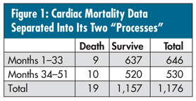
Figure 2 shows the generic structure of such data so that you can understand the needed statistical calculation.

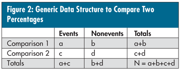
The following formula results in a chi-square statistic with 1 degree of freedom. The calculation looks worse than it is, but your statistical software package should have something akin to a “2 × 2 table chi-square analysis” or contained as an option within “cross-tabs” procedures. The interpretation, however, is quite simple:

  X_c² = N × [(absolute value ((a × d) - (b × c)) - N/2)] ² / [(a + b) × (c + d) × (a + c) × (b + d)], where N is the sum (a + b + c + d), the total number of observations.

So, for the data above:

  X_c² = 1,176 × [absolute value (4,680 - 6,370) - 588] ² / [(646) × (530) × (19) × (1,157)] = 0.190.

To test the obtained statistic from this analysis (and any future analysis using this technique) for statistical significance:

• For 5-percent risk or less (of declaring common cause as special cause): > 3.64,

• For 1-percent risk or less (of declaring common cause as special cause): > 6.63.

In other words, if your X_c² value is greater than these values, there is a good chance that the difference is real--the larger the value, the less your risk of declaring the difference as real when it isn’t. Obviously, with a value of 0.190 (which is much less than 3.64) for the bypass survival data, there is no evidence of a real difference.

Note: If you try to reproduce these results with your software package--which I highly recommend--it might give the X_c² value as 0.446 instead of 0.190. My calculation is technically the “correct” one because it adjusts for the fact that these data are “counts” and not continuous data. This is called the “correction for continuity” and is especially important if you have small sample sizes, which is not true in this case. Regardless, the interpretation is the same.

Now, let me change these data a bit in the table in figure 3, keeping the original data for months 1-33 and 98.6-percent survival rate. Note that I’ve changed the result of months 34-51 to 512 survivals out of 530 operations, which is a 96.6-percent survival (a decrease of 2%).

Applying the formula above yields an X_c² value of 4.35 (5.21 uncorrected), which, if one were to declare a difference, would have a risk of between 1 to 5 percent of being wrong. So, in this case, there would be good evidence that the survival rate had indeed gotten worse.

Then there is the problem of occurrences of very rare events, which invalidate this and the p-chart ANOM approximations. More about that next month.