A few days ago we received an email from a friend at a machine shop. He had just finished a process capability analysis for a critical feature (a runout on a cylindrical part) and was shocked by the output. The spreadsheet software he used showed him a process capability (Cpk) of 0.39 (see figure 1 below).
ADVERTISEMENT |
To put this in perspective, with a Cpk of 0.39, he should be seeing a nonconformance rate of between 12 percent and 24 percent, assuming a stable process and a normal distribution. However, he was actually experiencing a nonconformance rate close to zero. In fact, he hadn’t had any problems with runout as far back as he could remember.
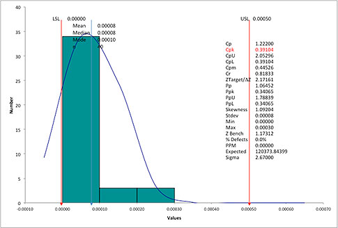
Why was the software telling him that his Cpk was 0.39 when the process was stable and located far away from the upper specification limit (USL)? The individuals control chart in figure 2 shows that the process is stable. So what was his real process capability?
Sources of errors
In general, we find two sources of error during process capability analysis:
1. The practitioner has violated one of the assumptions required for proper analysis. (For a list of assumptions, see “Pitfalls to Avoid with Cp, Cpk Process Capability Analysis.”)
2. The practitioner has not taken into consideration the “nature of the characteristic” being measured and has used an incorrect formula, or the software being used does not utilize the correct formula.
The nature of the characteristic
Runouts are specified with a single value: a not-to-exceed value. For example, the specification for runout was 0.0005 inches in this case. This means that the USL = 0.0005 in. But what is the lower specification limit (LSL)? And what is the nominal?
The LSL is obviously zero. In fact, zero is a hard limit; you can’t have a runout value less than zero. In addition, the nominal and the target value are also zero. In other words, in the ideal case, we should not have any runout.
Notice that the nominal is not midway between the USL and the LSL. Instead the nominal = LSL. These two facts, a hard LSL of zero, and a nominal = LSL, make runout a very special feature.
To make matters worse, runout data are often not normally distributed. Instead of a symmetrical distribution with a hump in the middle, we see a skewed distribution. A typical runout distribution will have a large number of values at or close to zero (the LSL), and fewer values closer to the USL.
Two challenges with runouts and other geometric dimensioning and tolerancing (GD&T) specifications
So now, we have identified two challenges with calculating Cpk for runouts:
1. The process is bounded and the nominal and target = LSL = zero
2. A non-normal distribution
Let’s deal with the first issue—a bounded process—first. Recall that Cpk is defined as min {Cpu, Cpl}. However, our goal is to have the process mean located near the target. In other words, the mean should be closer to the LSL and far from the USL. So our Cpk needs to be calculated as the distance from the USL to the process mean (i.e., Cpk = Cpu).
Therefore, the metric we use is Cpu. Assuming that the process is stable and the distribution is approximately normal (which we know is not exactly correct) we calculate:
Cpk = Cpu = (USL – Mean)/(3 * SigmaRSG),
where, SigmaRSG is the rational subgroup estimate of sigma (often incorrectly referred to as the short-term standard deviation), which in this case yields
Cpk = Cpu = 2.05.
The standard Cpk formula will work reasonably well for a process that is stable, mound shaped (normal), with a bilateral specification. However, if the process distribution is non-normal and bounded, then the standard formula may not yield very realistic results. So let’s consider the impact of a non-normal distribution on the Cpk calculation. Once again we assume the process is stable.
There are two approaches to estimating process capability in this case:
1. Model the observed data distribution and estimate the nonconformance rate from the fitted model.
2. Use capability indices designed to analyze non-normal process distributions.
The modeling and curve-fitting approach may provide a more realistic estimate of the nonconformance rate than the standard formula for non-normal data. However, we don't think the modeling approach is a realistic solution for many small companies as they may not have the technical expertise nor the software necessary to perform the analysis. Hence, the other option is to try and address this problem with a simple metric that would still provide a reasonably accurate assessment of process capability. The metric we feel offers a resonable choice is the ISO Technical Committee (TC) 69—”Application of statistical methods” formula.
Cpk = min{Cpu, Cpl},
Cpu = (USL - Median)/(p(0.99865) - Median)
Cpl = [(Median - LSL)/(Median - p(0.00135))]
The percentile points p(0.99865) = UCL and p(0.00135) = LCL correspond to the tail areas of a normal distribution with three sigma limits.
Using the ISO/TC 69 formula, we find that the Cpk for our data is 1.91 vs. 2.05 when we had assumed normality and use the mean rather than the median.
Keep in mind
Mean vs. the median: As a reminder, the mean is influenced by outliers in the data set. Therefore, when we deal with skewed (non-normal) distributions, we use the median as the measure of central tendency as it is not as influenced by outliers in the data set.
Other non-normal metrics: There are other estimators that are designed to handle non-normal distributions including Cnpk, or Cp(q) that appear to provide similar results.
Comments
Calculating Cpk when there is no LSL
In this example, there is no LSL, just an upper specification limit (USL).In the QI Macros, if you specify the USL with no LSL, Cpk=Cpu would be 2.05 instead of 0.39.
We could substitute median for the average to get 1.91, but in either case Cpk is much greater than 1.66 (5 sigma) and close to 2.0 (6 sigma).
Yes, in this case a median will be a better measure of central tendency, but do we really need a micrometer or is this yardstick good enough? While Average could easily be changed to Median in the QI Macros Histdata worksheet, would it tell a better story?
The QI Macros do have a true position Cp Cpk template for GD&T calculations (using variation both from X and Y coordinates).
KNOWWAREMAN
Why even bother?
Why are we in the Quality profession still espousing this psuedo statistic?
All these girations to calculate a single number that is simply not informative or actionable.
What does the index tell us that the run chart (multi-var or control chart) doesn't? nothing.
We must start with it to determine stability. We must go back to it to begin to understand how to improve the process. We must go to it to understand if the index is even reasonably correct...
BDANIELS
Mononumerosis
I couldn't agree more. Capability indicies are one of the most abused statistics. Management likes them because they boil everything down to one number. I had a professor term this mononumerosis.
For a very good discussion on capability indices, refer to the January 2002 issue of ASQ "Journal of Quality Technology." The entire issue is dedicated to this subject.
Cpk calculations
I couldn't agree more with BDaniels. I understand the authors' reply that sometimes these are "required." Yet, when we perfunctorily make these calculations without understanding the meaning or purpose of the number, we do ourselves and others little good. Fine report the number, but then also report what is useful and meaningful and actionable. Maybe people will eventually drop the useless information requirement.
The authors identify that IF the formula requires assumptions, then common errors will often be due to violations of those assumptions.
But, the formula in itself does not require either stability or normality--nor does the meaning of the concept. These are assumptions added by people who thought they were necessary. They can be circumvented, the authors suggest one way, by understanding the meaning of process capability. The meaning--at least the one I would want to use--is the probability of meeting specification(s).
This is the meaning I give it regardless of the index. Different process capability indices differ only in the conditions under which that probability is determined.
But since we can only estimate the probability for some of these conditions, e.g., what is the "best" the process is capable of?--then we need to understand whether adding assumptions make those estimates better, when, and how? Sometimes the assumptions are neither useful nor necessary.
Just as we should recognize when Cpk is useful/necessary or not, we should also recogize when stability and normality assumptions are useful/necessary or not.
Add new comment