Calculating Reliability and Confidence

How to generate an OC curve based on sample size and number of rejects

Published: Monday, November 18, 2019 - 13:03

It has been a while since I have written about statistics, and I get asked a lot about a way to calculate sample sizes based on reliability and confidence levels. So today I am sharing a spreadsheet that generates an operating characteristic (OC) curve based on your sample size and the number of rejects. The spreadsheet (there's a link to it at the end of this article) should be straightforward to use. Just enter your own data in the required yellow cells.

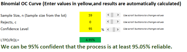
A good rule of thumb is to use a 95-percent confidence level, which also corresponds to 0.05 alpha. The spreadsheet will plot two curves. One is the standard OC curve, and the other is an inverse OC curve. The inverse OC curve has the probability of rejection on the y axis, and the percent conforming on the x axis. These correspond to confidence level and reliability, respectively.

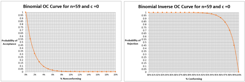
I will discuss the OC curve and how we can get a statement that corresponds to a reliability/confidence level from the OC curve.

The OC curve is a plot between percent nonconforming, and probability of acceptance. The lower the percent nonconforming, the higher the probability of acceptance. The probability can be calculated using binomial, hypergeometric or Poisson distributions. The OC curve shown is for n = 59, with 0 rejects. It is calculated using binomial distribution.

The producer’s risk is the risk of good product getting rejected. The acceptance quality limit (AQL) is generally defined as the percent of defectives that the plan will accept 95 percent of the time (i.e., in the long run). Lots that are at or better than the AQL will be accepted 95 percent of the time (in the long run). If the lot fails, we can say with 95-percent confidence that the lot quality level is worse than the AQL. Likewise, we can say that a lot at the AQL that is acceptable has a 5-percent chance of being rejected. In the example, the AQL is 0.09 percent.

The consumer’s risk, on the other hand, is the risk of accepting bad product. The lot tolerance percent defective (LTPD) is generally defined as percent of defective product that the plan will reject 90 percent of the time (in the long run). We can say that a lot at or worse than the LTPD will be rejected 90 percent of the time (in the long run). If the lot passes, we can say with 90-percent confidence that the lot quality is better than the LTPD (i.e., the percent nonconforming is less than the LTPD value). We could also say that a lot at the LTPD that is defective has a 10-percent chance of being accepted.

The vertical axis (y axis) of the OC curve goes from 0 percent to 100 percent probability of acceptance. Alternatively, we can say that the y axis corresponds to 100 percent to 0 percent probability of rejection. Let’s call this confidence.

The horizontal axis (x axis) of the OC curve goes from 0 percent to 100 percent for percent nonconforming. Alternatively, we can say that the x axis corresponds to 100 percent to 0 percent for percent conforming. Let’s call this reliability.

We can easily invert the y axis so that it aligns with a 0 to 100-percent confidence level. In addition, we can also invert the x axis so that it aligns with a 0 to 100-percent reliability level. This is shown below.

What we can see is that, for a given sample size and defects, the more reliability we try to claim, the less confidence we can assume. For example, in the extreme case, 100-percent reliability lines up with 0-percent confidence.

I welcome readers to play around with the spreadsheet. I am very interested in your feedback and questions. Click here to download the spreadsheet. I have written several articles on reliability and confidence. Check this post and this post for additional details.

First published Oct. 19, 2019, on Harish's Notebook.

About The Author

Harish Jose

Harish Jose has more than seven years experience in the medical device field. He is a graduate of the University of Missouri-Rolla, where he obtained a master’s degree in manufacturing engineering and published two articles. Harish is an ASQ member with multiple ASQ certifications, including Quality Engineer, Six Sigma Black Belt, and Reliability Engineer. He is a subject-matter expert in lean, data science, database programming, and industrial experiments, and publishes frequently on his blog Harish’s Notebook.