by Davis Balestracci
The current design of experiments (DOE) renaissance seems to favor factorial designs and/or orthogonal arrays as a panacea. In my 25 years as a statistician, my clients have always found much more value in obtaining a process "road map" by generating the inherent response surface in a situation. It's hardly an advanced technique, but it leads to much more effective optimization and process control.
The following are typical curricula for DOE in Six Sigma programs. The main topics for many basic DOE courses include:
• Full and fractional factorial designs
• Screening designs
• Residual analysis and normal probability plots
• Hypothesis testing and analysis of variance
Main topics for many advanced DOE courses include:
• Taguchi signal-to-noise ratio
• Taguchi approach to experimental design
• Response-surface designs (e.g., central composite and Box-Behnken)
• Hill climbing
• Mixture designs
No doubt these are all very interesting, but people don't need statistics; they need to solve their problems. A working knowledge of a good, basic experimental design software package containing easy-to-use, appropriate regression diagnostics is far more valuable and negates the need to teach several of the above topics.
This article will use a relatively common scenario to demonstrate sound experimental design philosophy and its flexibility as well as a "takeaway" I consider a bread-and-butter design tool for any quality practitioner. It will also show you, to paraphrase Yogi Berra, that "90 percent of statistics is half planning."
Let's consider a production process where the desired product immediately decomposes into a pesky, tarry byproduct. The process is currently averaging approximately 15 percent tar, and each achievable percent reduction in this tar is equivalent to more than $1 million in annual savings.
Process history has shown three variables to be crucial in controlling the process. The variables and chosen regions for experimentation are temperature, 55-65° C; copper sulfate (CuSO4), 26-31 percent; and excess nitrite (NO2-), 0-12 percent. Any combination of the three variables within these ranges would represent a safe and economical operating condition. The current operating condition is in the midpoint of these ranges.
For the purposes of experimentation only, the equipment is capable of operating in the following ranges if necessary: temperature, 50-70° C; CuSO4, 20-35 percent; and excess NO2-, 0-20 percent.
Suppose you had a budget of 25 experiments.
• Where should the process operate (i.e., where should the three variables be set)?
• What percent tar would you expect?
• What's your best estimate of the process variation (i.e., tar ± x percent)?
This is the scenario I use to introduce my experimental design seminars. I form groups of three to four people to simulate experimental conditions... and get as many different answers for the optimum as there are groups in the room, and just as many strategies (and number of experiments run) for reaching their conclusions.
General observations:
• Most try holding one to two of the variables constant while varying the third and then optimizing around their best result.
• Each experiment seems to be run based only on the previous result.
• Some look at me smugly and do a 23 factorial design (and, generally, get the worst answers in the room).
• Some run more than the allotted 25 experiments.
• Some go outside of the established variable ranges.
• Some look at me like I'm nuts when I tell them:
--Repeating a condition uses up one of their experiments.
--They should repeat their alleged optimum (and it counts as an experiment…).
• I'm accused of horrible things when the repeated condition gets a different answer (sometimes differing by as much as 11-14 percent). I simply ask, "If you run a process at the same conditions on two different days, do you get the same results?"
Because of the above observations:
• I'm sometimes told the "process is out of control," so there's no use experimenting.
• Most estimates of process variability are low.
• Groups have no idea how to present results in a way that would "sell" them to management.
• The suggested optimal NO2 - settings are all over the range of 0-12 (and, by the way, that variable is modeled to have no effect).
It's not as simple as declaring, "We want to run an experiment." The presence of natural process variation clouds the issue, so we must first consider this question: Is the objective to optimize or establish effects?
Given any situation, there's an inherent response surface--i.e., the "truth"--that one is trying to model and map. Any experimental result represents this true response, clouded, unfortunately, by the common-cause variation in the process.
The true surface (called a "contour plot") of the tar scenario is shown in figure 1. (The NO2 - variable has zero effect.) My simulator generates this true number along with a random, normally distributed error that has a standard deviation of four. Note that any combination of temperature and copper sulfate concentration allows one to read the corresponding resulting tar formation from the contours, and that tar is minimized at 65° C and approximately 28.8 percent CuSO4.
Figure 1: True Tar Response Surface
It can be generated either directly in the case of a high state of process knowledge (i.e., "optimize"), or established sequentially for a low state of process knowledge once critical variables and their important ranges are found (i.e., "establish effects").
From calculus, any function can be modeled as an infinite power series. Response surface DOE's objective is to model the current situation by a power series truncated after the quadratic terms--a quadratic "French curve." In the current case of our three variables:
Y=B0 + B1x1 + B2x2 + B3x3 + B12x1x2 + B13x1x3 + B23x2x3 + B11x12 + B22x22 + B33x32
So, what design(s) gives one the best estimates of these "B" coefficients? It's like building a tabletop: Where does one place the legs? I often see people, in essence, running large numbers of experiments along the "diagonal" of the table, when four well-placed experiments at the corners would actually be more efficient.
The first two designs that follow consider the "optimize" objective and represent a damn-the-torpedoes approach. You just want to optimize your process and get on with life.
The third design demonstrates the "establish effects" objective and its inherent sequential approach. This is a low "state of the knowledge" strategy where time is needed to identify critical variables and map the interesting design subspace.
If this were a relatively mature process where these three variables had evolved as key process controllers, and if DOE was a new concept to the organization and a quick success was needed, I'd use the design shown in figure 2. It's known as a three-variable Box-Behnken design with 15 runs. It's shown in its coded (i.e., geometric) form on the left and actual variable settings on the right (-1 represents the low setting of the variable, and +1 represents the high setting). It's structured to run all possible 2x2 factorial designs for the three possible independent variable pairings (i.e., x1 and x2, x1 and x3, x2 and x3) while holding the other variable at its midlevel.
These 15 experiments should be run randomly. Note that the data point with each variable at its midpoint (i.e., center point) is run three separate times. These replications, called a "lack of fit" test, are key to checking whether the region chosen is too large to be approximated by a quadratic equation.
Lack of fit is only one of four diagnostics of the generated quadratic equation. It's beyond this article's scope to teach the appropriate regression analysis and its diagnostics. However, briefly, the residuals (i.e., actual values minus the predicted values) contain all of the information needed to diagnose the model fit.
So, besides the above lack-of-fit test:
• A residuals-vs.-predicted values plot, which should look like a shotgun scatter, might indicate the need for a transformation of the response (e.g., viscosity).
• A normal plot of the residuals tests the implicit assumption of normality for least squares regression.
• A run chart of the residuals in the order in which the experiments were run checks whether an outside influence crept in during the experiment.
For my money, this should be a "bread-and-butter" design for all quality practitioners in a high "state of knowledge" situation needing some fast answers. Think about it: You could generate a response surface by the efficient use of only 15 experiments.
Note that, in contrast to the Box-Behnken, it's usually not possible to optimize a process using, in this case, a 23 factorial experiment. A factorial experiment can only get the linear terms and interaction terms of the underlying equation, not the quadratic terms. Optimizing via the eight experimental runs from the factorial design can only lead to one of the cube's corners--which in this case would be incorrect. As will be shown, should a more sequential strategy (to establish effects) be chosen, adding center points (i.e., all variables at their midpoints) to a standard factorial design allows one to test whether further experimentation is indeed even needed for optimization, which would build on the current design. (The ability to optimize solely with a factorial design tends to be the exception.)
What's another possibility for our situation? To use the statistician's favorite answer, "It depends." Another design many of you have heard about is the central composite design. In this situation, it would be set up as in the table in figure 3.
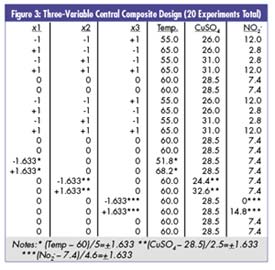
It's a factorial design augmented by an additional block of experiments (called "star points"), where each individual variable is taken to two further extremes while the other two are held at their midpoints. The subsequent response surface will be most valid for variables in their [-1, 1] coded ranges.
You'll also see that it takes 20 experimental runs in this case and creates the potential problem of dealing with five levels for each variable. It has happened often enough in my experience to mention that, occasionally, this additional star-point block of experiments causes problems with the quadratic approximation because the region is extended beyond its reasonable limits, as indicated by the lack-of-fit test.
It depends. How well do you know your process and, once again, is your objective to establish effects or optimize?
For example, maybe the objective of initial experimentation was to see whether all three variables were necessary before proceeding with generating the response surface. The naive approach would be to run an unreplicated 23 factorial design.
Now, you'll notice that the central composite design does just that; however, one has committed up front to running the entire design and must therefore plot the resulting equation regardless of effects.
Excuse me while I digress to two crucial topics:
It's not as simple as running a 23 factorial (because you have three variables) and "picking the winner." In this case, running eight experiments could detect only a variable's effect if it made a difference of approximately 11 percent tar when set at its upper range, as opposed to being set at its lower range (dependent on the process standard deviation of ±4). Repeating the entire experiment--16 runs plus center points--now allows you to detect a difference of 8 percent.
If you're going to run 16 experiments (plus a few center points), did you know that you could add up to five more variables (i.e., eight variables total) to see whether their effects are significant? (For more on screening designs, see R. M. Moen, T. W. Nolan and L. P. Provost, Quality Improvement Through Planned Experimentation, Second Edition, McGraw-Hill, 1999.) This strategy also allows one to make important decisions regarding noncontinuous variables (i.e., catalyst A vs. catalyst B, with no center point possible) before continuing to the map.
Then there are "interactions," which are the rule rather than the exception. From the tar response surface, note the difference in the effect of temperature at the low level of CuSO4, where tar can vary from 12 percent at 65° C to more than 50 percent at 55° C, vs. the high level of CuSO4, where the percent tar is relatively constant around 10 percent, regardless of the temperature. Because of the concept of interactions, ignoring other variables puts you at the mercy of their current settings. In other words, if you decide to experiment in the future on those variables currently held constant, it could possibly (and would most probably) invalidate the results of your current experiment.
Rules of thumb:
• Sixteen factorial experiments are an efficient number to run.
• Be inclusive with the independent variables, especially when they amount to eight or fewer.
We were asking the question, "Are three variables necessary?"
Scenario 1 : Suppose one did repeat a 23 factorial design (with ranges of 55-65° C for temperature, 26-30 percent for CuSO4 and 0-12 percent for NO2 -) and discovered that the NO2 - variable was indeed not significant. How would one proceed?
You'd run the star-point block of experiments as seen in figure 4 (in random order), probably setting NO2 - at zero. Because of the geometry of the situation (i.e., repeated factorial cube), the star-point settings are now ±2 instead of ±1.633. (Note that you'll have now run 27 experiments total.)

These data would build on your previous data, all of which would be used in the analysis.
Scenario 2: Suppose that NO2 - was significant? Because the initial objective was to see whether it was indeed necessary, the lower level of NO2 - has already been set to zero, unlike some experiments that anticipate zero being the low star-point setting. In this case, it would now be impossible to have the coded "-1.633" setting for the lower star point because negative NO2 - is impossible. Experience has shown that one should use its lower limit (i.e., 0) as the lowest star-point setting and repeat that condition for the "tabletop" stability needed in the equation generation and/or analysis. This replicate would be independently randomized into the design, as shown in figure 5.
What seemed like a relatively straightforward scenario turned out to have a lot of potential approaches for its solution. However, good experimentation relies on the process of asking the appropriate questions to define clear objectives beyond the typical, "We need to run an experiment."
Davis Balestracci is a member of the American Society for Quality and past chair of its statistics division. Visit his Web site at www.dbharmony.com.
|