SPCTool




	How Much Data Do I Need? The relationship between degrees of freedom and the coefficient of variation is the key to answering the question of how much data you need. by Donald J. Wheeler
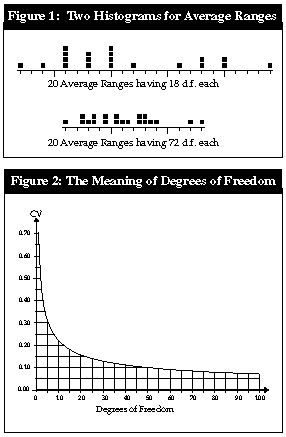
	How much data do I need to use when I compute limits?" Statisticians are asked this question more than any other question. This column will help you learn how to answer this question for yourself. Implicit in this question is an intuitive understanding that, as more data are used in any computation, the results of that computation become more reliable. But just how much more reliable? When, as more data become available, is it worthwhile to recompute limits? When is it not worthwhile? To answer these questions, we must quantify the two concepts implicit in the intuitive understanding: The amount of data used in the computation will be quantified by something called "degrees of freedom," and the amount of uncertainty in the results will be quantified by the "coefficient of variation." The relationship between degrees of freedom and the coefficient of variation is the key to answering the question of how much data you need. The terminology "degrees of freedom" cannot be explained without using higher mathematics, so the reader is advised to simply use it as a label that quantifies the amount of data utilized by a given computation. The effective degrees of freedom for a set of control limits will depend on the amount of data used and the computational approach used. For average and range charts (X-bar and R charts), where the control limits are based upon the average range for k subgroups of size n, the degrees of freedom for the limits will be: d.f. ~ 0.9k(n1). For example, in April's column, limits were computed using k = 6 subgroups of size n = 4. Those limits could be said to possess: 0.9 (6) (3) = 16.2 degrees of freedom. For average and standard deviation charts (X-bar and s charts), where the control limits are based on the average standard deviation for k subgroups of size n, the degrees of freedom for the limits will be: d.f. ~ k(n1) 0.2(k1). In my April column, if I had used the average standard deviation to obtain limits, I would have had: (6) (3) 0.2 (5) = 17 degrees of freedom. As will be shown below, the difference between 16 d.f. and 17 d.f. is of no practical importance. For XmR charts, with k subgroups of size n = 1, and limits based on the average moving range, the degrees of freedom for the limits will be: d.f. ~ 0.62 (k1). In my March column, I computed limits for an XmR chart using 20 data. Those limits possessed: 0.62 (19) = 11.8 degrees of freedom. The better SPC textbooks give tables of degrees of freedom for these and other computational approaches. However, notice that the formulas are all functions of n and k, the amount of data available. Thus, the question of "How much data do I need?" is really a question of "How many degrees of freedom do I need?" And to answer this, we need to quantify the uncertainty of our results, which we shall do using the coefficient of variation. Control limits are statistics. Thus, even when working with a predictable process, different data sets will yield different sets of control limits. The differences in these limits will tend to be small, but they will still differ. We can see this variation in limits by looking at the variation in the average ranges. For example, consider repeatedly collecting data from a predictable process and computing limits. If we use k = 5 subgroups of size n = 5, we will have 18 d.f. for the average range. Twenty such average ranges are shown in the top histogram of Figure 1.

If we use k = 20 subgroups of size n = 5, we will have 72 d.f. for the average range. Twenty such average ranges are shown in the bottom histogram of Figure 1. Notice that, as the number of degrees of freedom increase, the histogram of the average ranges becomes more concentrated. The variation of the statistics decreases as the degrees of freedom increase.

A traditional measure of just how much variation is present in any measure is the coefficient of variation, which is defined as:

CV = standard deviation of measure/mean of measure

Examining Figure 1, we can see that as the degrees of freedom go up, the coefficient of variation for the average range goes down. This relationship holds for all those statistics that we use to estimate the standard deviation of the data. In fact, there is a simple equation that shows the relationship. For any estimate of the standard deviation of X:

CV = 1/sq.rt.(2d.f.)

This relationship is shown in Figure 2.

So just what can you learn from Figure 2? The curve shows that when you have very few degrees of freedom -- say less than 10 -- each additional degree of freedom that you have in your computations results in a dramatic reduction in the coefficient of variation for your limits. Since degrees of freedom are directly related to the number of data used, Figure 2 suggests that when we have fewer than 10 d.f., we will want to revise and update our limits as additional data become available.

The curve in Figure 2 also shows that there is a diminishing return associated with using more data in computing limits. Limits based upon 8 d.f. will have half of the variation of limits based upon 2 d.f., and limits based upon 32 d.f. will have half of the uncertainty of limits based upon 8 d.f. Each 50-percent reduction in variation for the limits requires a four-fold increase in degrees of freedom. As may be seen from the curve, this diminishing return begins around 10 degrees of freedom, and by the time you have 30 to 40 d.f., your limits will have solidified.

So, if you have fewer than 10 degrees of freedom, consider the limits to be soft, and recompute the limits as additional data become available. With Shewhart's charts, 10 degrees of freedom require about 15 to 24 data. You may compute limits using fewer data, but you should understand that such limits are soft. (While I have occasionally computed limits using as few as two data, the softest limits I have ever published were based on four data!)

When you have fewer than 10 d.f. for your limits, you can still say that points which are comfortably outside the limits are potential signals. Likewise, points comfortably inside the limits are probable noise. With fewer than 10 d.f., only those points close to the limits are uncertain.

Thus, with an appreciation of the curve in Figure 2, you no longer must be a slave to someone's arbitrary guideline about how much data you need. Now you can use whatever amount of data may be available. You know that with fewer than 10 d.f., your limits are soft, and with more than 30 d.f., your limits are fairly solid. After all, the important thing is not the limits but the insight into the process behavior that they facilitate. The objective is not to get the "right" limits but rather to take the appropriate actions on the process.

So use the amount of data the world gives you, and get on with the job of separating potential signals from probable noise.

About the author

Donald J. Wheeler is an internationally known consulting statistician and author of Understanding Variation: The Key to Managing Chaos and Understanding Statistical Process Control, 2nd Edition.



	e-mail Quality Digest

Please contact our Webmaster with questions or comments.