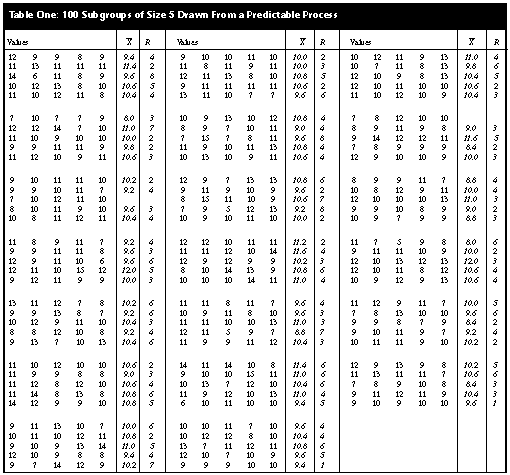
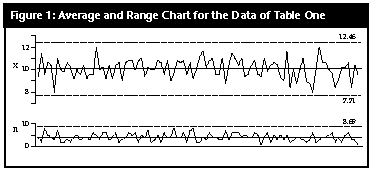
Based on these data, the natural process limits would be computed as: X= ± 3R-/d2 = 10.084 ± 3 (1.767) = 4.78 to 15.39 meaning that we should expect process values that range from 5 to 15. If the specification limits for this process are 3 to 17, then we will have a process in the ideal state -- both predictable and conforming. With these specification limits and the summary statistics from the control chart, the capability ratio for this bead board process would be: Cp = (USL-LSL)/6Sigma(X) = (17-3)/(6.0)(1.767) = 1.32 With a grand average of 10.084, the centered capability ratio is: Cpk = (USL-X=)/3Sigma(X) = (17-10.084)/(3.0)(1.767) = 1.30 Today, many customers ask for centered capability ratios of 1.33 or greater. While this process is close, it does not quite meet this magic value. The calculations above are based on 500 data, and we seldom wait until we have so much data to compute the capability ratios. In most cases, capabilities are computed occasionally, or periodically, using 50 or fewer values. So we shall divide our 100 subgroups into blocks of 10 subgroups each and compute the Cpk value for each block. Ten subgroups of size 5 will yield estimates of dispersion with about 36 degrees of freedom, which is commonly considered to be satisfactory. Subgroups 1 to 10: Grand average = 10.08, average range = 4.0, and Sigma(X) = 4.0/2.326 = 1.720 The centered capability ratio is: Cpk = (17.0-10.08)/(3.0)(1.720) = 1.34 A good capability ratio -- our customer will be pleased with this. Subgroups 11 to 20: Grand average = 9.98, average range = 3.9, and Sigma(X) = 3.9/2.326 = 1.677 The centered capability ratio is: Cpk = (9.98-3.0)/(3.0)(1.677) = 1.39 Congratulations, the capability ratio got better. Subgroups 21 to 30: Grand average = 10.12, average range = 4.5, and Sigma(X) = 4.5/2.326 = 1.935 The centered capability ratio is: Cpk = (17.0-10.12)/(3.0)(1.935) = 1.19 What happened to cause the capability ratio to drop? Subgroups 31 to 40: Grand average = 10.24, average range = 4.2, and Sigma(X) = 4.2/2.326 = 1.806 The centered capability ratio is: Cpk = (17.0-10.24)/(3.0)(1.806) = 1.25 This capability ratio is still not good enough -- we must do better. Subgroups 41 to 50: Grand average = 10.10, average range = 4.9, and Sigma(X) = 4.9/2.326 = 2.107 The centered capability ratio is: Cpk = (17.0-10.10)/(3.0)(2.107) = 1.09 This is worse than before, and the third value is below 1.33 -- things had better improve or else! Subgroups 51 to 60: Grand average = 10.42, average range = 3.9, and Sigma(X) = 3.9/2.326 = 1.677 The centered capability ratio is: Cpk = (17.0-10.42)/(3.0)(1.677) = 1.31 Well, this is better, but our customer is asking for 1.33 or greater. Subgroups 61 to 70: Grand average = 10.30, average range = 4.7, and Sigma(X) = 4.7/2.326 = 2.021 The centered capability ratio is: Cpk = (17.0-10.30)/(3.0)(2.021) = 1.11 You were supposed to be improving -- what is going on here? Subgroups 71 to 80: Grand average = 10.06, average range = 3.8, and Sigma(X) = 3.8/2.326 = 1.634 The centered capability ratio is: Cpk = (17.0-10.06)/(3.0)(1.634) = 1.42 At last -- send these data to our customer. Subgroups 81 to 90: Grand average = 9.88, average range = 3.5, and Sigma(X) = 3.5/2.326 = 1.505 The centered capability ratio is: Cpk = (9.88-3.0)/(3.0)(1.505) = 1.52 Excellent capability ratio. Good work. Subgroups 91 to 100: Grand average = 9.66, average range = 3.7, and Sigma(X) = 3.7/2.326 = 1.591 The centered capability ratio is: Cpk = (9.66-3.0)/(3.0)(1.591) = 1.40 Why is this value slipping? Of course, the real answer is that we are not slipping. The process was not getting worse, nor was it getting better. But our statistics were changing from block to block even though the process remained the same, and these changes were reflected in the centered capability ratio values computed. If we placed these 10 centered capability ratios on an XmR chart, we would get Figure 2. |