Please Don't Feed Averages
Michael J. Cleary, Ph.D.
mcleary@qualitydigest.com
The behavior of averages can
be as fascinating as that of animals. Hartford Simsack,
intrepid quality manager for Greer Grate & Gate, sometimes
thinks of himself as a visitor to the zoo, watching his
averages and trying to anticipate what, to him, was always
a complete surprise in the behavior of data. "I never
know if this is going to turn out to be a normal distribution
or not," he told his mentor, Dr. Stan Deviation.
Deviation cleared his throat and reminded Simsack yet
again that one of the keys to predicting the shape of the
averages lies in sample size. Regardless of the distribution
shape of the parent population, the distribution of sample
means from that population will follow a normal distribution
if the sample size is, for example, five. You'll remember
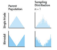
that in July's column, Deviation demonstrated a simulation
model with 1,000 samples of the sizes one and two from two
populations to demonstrate the shape of the distributions
from both. Unfortunately, Simsack doesn't recall either
the column or his mentor's lecture about this point.
The charts below demonstrate the concept:
Simsack can never quite get his mind around this concept.
Unfortunately for him, however, his boss can and often asks
him for an explanation. Rock DeBote not only wants an answer,
but he also wants to understand the concept well enough
so that he can derive his own understanding. After his conversation
with Deviation, Simsack is quick to respond to nearly every
question about distribution, "It all depends on sample
size." DeBote isn't content with this superficial answer
and presses Simsack for the statistical concept responsible
for this outcome.
"It's the central limit theorem," Simsack responds
smugly.
This is a term with which he's familiar, and it's what
comes immediately to his lips. Is he correct?
Amazingly, Simsack drops the right term this time. The
behavior of averages in this case is indeed related to the
central limit theorem. In June's column, we examined the
rules for determining out-of-control situations, noting
that the important caveat is not which set of rules to use
but rather to use them consistently.
Some disagree about whether the central limit theorem
is needed as a basis for these sets of rules. Some note
that Walter Shewhart never cited the central limit theorem
in his seminal work, Economic Control of Quality of Manufactured
Products (D. Van Nostrand Co. Inc., 1931). In my university
experience, students have proved able to understand the
central limit theorem once they grasp the difference between
averages (X) and individual values (Xi) and the ways in
which the two behave.
The easiest way to demonstrate the central limit theorem
is by using PQ Systems' Quality Gamebox. As noted above,
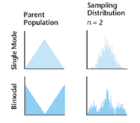
if one takes 1,000 samples from a known population, then
creates a distribution of sample means (n = 2), that distribution
will be different from the population. Using Quality Gamebox,
but taking a sample size of five, the following results
ensue:
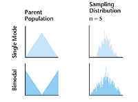
The most interesting result lies in the appearance of
the distribution of sample means from the bimodal parent
population. This clearly demonstrates the application of
the central limit theorem:
 The mean of the sample means' distribution is close to the
population's mean.
The mean of the sample means' distribution is close to the
population's mean.
The shape of the distribution of sample means is normal-looking.
The sample means' distribution variability is less than
the parent population.
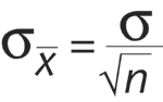
Note: It's equal to the standard deviation of the population
divided by the square root of the size of the sample used
to create the distribution of sample means:
Once one understands the central limit theorem, the three
basic rules for an out-of-control situation are easily derived.
The most commonly accepted out-of-control rules were derived
directly from the central limit theorem:
Any point outside the control limits is out of control.
The probability that this will happen when a system is in
control is 0.0023. A point appearing outside the control
limits is a signal that the process is out of control.
Runs above the mean or below the mean equal 0.0073 and indicate
an out-of-control signal. If seven averages in a row become
larger or slower, this is called "runs up" or
"runs down." Such an occurrence is unlikely for
a process that is in control, so this would be considered
a signal for an out-of-control situation.
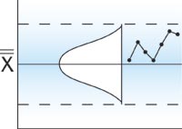
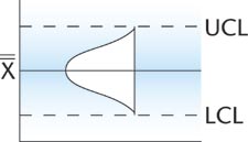
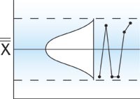
Because the distribution of sample means (for sample size
of five or more) forms a normal distribution, one would
expect the X to reflect that pattern. A pattern such as
those below suggests the process is out of control.
Michael J. Cleary, Ph.D., is a professor emeritus at Wright
State University and founder of PQ Systems Inc. Letters
to the editor regarding this column can be e-mailed to letters@qualitydigest.com.
|