I Hate Bar Graphs--Part 2
One day, I walked into a hospital administrator’s office and saw the chart in figure 1 on his desk. What is this obsession with bar graphs and presenting multiple-year data in this format? I can just hear some of you saying, "Well… er… uh… seasonality!"
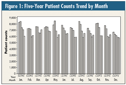
In plotting these 60 observations in their time order, there are two distinct breaks: January of year three and four, due to new employee health insurance benefits kicking in. But regardless of the year and despite these January shifts, is there a consistent, predictable pattern of monthly patient behavior every year?
Given the fact that the distinct breaks happen in January, there’s some justification to use analysis of variance (ANOVA), which yields the table in figure 2.
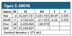
Before proceeding further with this model/analysis, it’s necessary to use the four graphical diagnostics described in my February 2006 Quality Digest article about design of experiments ("Using Design of Experiments as a Process Road Map"), all of which were satisfied.
Because both "year" and "month" p-values are < 0.05, the questions become: Which years? Which months?
The analysis of means (ANOM) used to compare year-by-year and month-to-month "seasonality" are shown in figure 3. Three standard deviations are used for the limits. (See last month’s column on ANOM limits.)
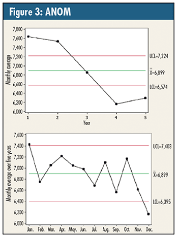
The top graph confirms what the time plot showed: significant shifts in January of years three and four. If the "plot of the residuals in time order showing no pattern" diagnostic had failed, it would have invalidated the "significant process shift at January" model.
The bottom graph compares the monthly averages. The underlying structure of the standard deviation (i.e., the square root of the "error" term MS in the ANOVA) has inherently "adjusted" for these yearly process shifts so that they don’t interfere with this monthly comparison.
Figure 4 provides a summary table of the twelve monthly averages.

Only because the ANOVA gave a significant result for "month" can one now calculate what is statistically called the least significant difference (LSD), used to interpret the differences in monthly averages. I won’t go through the mechanics because that would distract from the purpose of this column, but suffice it to say that the LSD in this case is 479.
The human tendency is to focus arbitrarily on the largest differences, so there’s another number that adds an element of conservatism and balance. Theoretically, with 12 means, there are 66 pairwise comparisons. So, utilizing the Studentized range to compare any two months, this difference becomes 821.
What do you think?
Next month, I’ll show you how "boring" SPC can shed some further insights to give a wonderful final graphical summary of these data… which, by the way, will differ from the preliminary seasonality analysis above.
Davis Balestracci is a member of the American Society for Quality and past chair of its statistics division. Visit his Web site at www.dbharmony.com
|