There’s a lot of buzz about “data analytics”—mining huge data sets to discover invisible patterns of customer behavior that can be leveraged to maximize sales. But I’ve found that few people know how to mine the hidden improvement projects from existing “small data” using Excel’s PivotTables.

Over the years, I have used Excel PivotTables on projects that:
• Saved $20 million in postage expenses
• Save $16 million in adjustment costs
• Reduced order errors in a cell phone company from 17 to 3 percent in just four months, saving $3 million a year in rework
• Reduced denied insurance claims in a health care system that saved $5 million a year with simple process changes that could be implemented immediately

Using PivotTables for data mining is the key to finding multimillion-dollar improvement projects.

What small data look like

Almost every business I’ve ever consulted with has data about defects, mistakes, and errors in an Excel spreadsheet. These data are a line-by-line, date-by-date, account of the origin and type of defect. For packaging defects on a production line, the data might look like this:

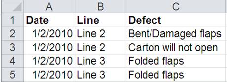
Figure 1: Example of data on packaging defects on a production line

For lost time analysis, the data might look like this:

Figure 2: Example of data for lost time analysis

Or for hospital denied charges, they might look like this:

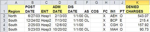
Figure 3: Example of data for hospitals’ denied charges

Turning data into improvement projects

To turn these kind of data into something that can be charted requires the use of Excel PivotTables. PivotTables can:
• Count the occurrences of a keyword, phrase, or number
• Sum or average numbers
• Turn raw data into knowledge
• Help drill down into mounds of data

Setting up your spreadsheet

PivotTables can get cranky if you don’t follow these guidelines:
• Each column must have a unique heading.
• No blank columns
• Cells with no data should be left blank (otherwise they will be counted).
• Data should be consistent (e.g., Colorado vs. Colo).
Tip: Most data require some cleanup before analysis.

Packaging defects example

To create a PivotTable using packaging defects, simply click on any cell within the range you want to summarize, and then select Insert PivotTable as shown in figure 4a (Excel 2007–2010). Excel will automatically select the data for you, as shown in figure 4b.

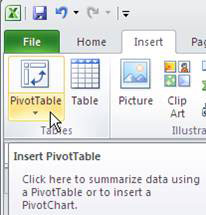
Figure 4a: Select Insert PivotTable in Microsoft Excel

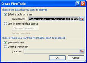
Figure 4b:  Excel selects data from cells to create a PivotTable

Then, click OK, and Excel will provide a template to organize the data, as shown in figures 5a and 5b.

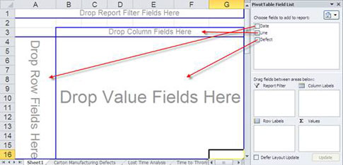
Figure 5a: Organizing data by dragging and dropping data fields onto the Excel template

You can then drag and drop fields onto the template as in figure 5a above or as shown in figure 5b below.

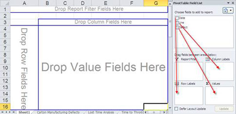
Figure 5b: Organizing data by dragging and dropping data fields onto PivotTable layout areas

Excel’s PivotTable will summarize the data, as seen in figure 6.

Figure 6: Packaging defect data are summarized and displayed in a PivotTable

Now we can draw a control chart of defects by day and a Pareto chart by line (see figures 7 and 8).

Figure 7: Control chart of packaging defects data by date

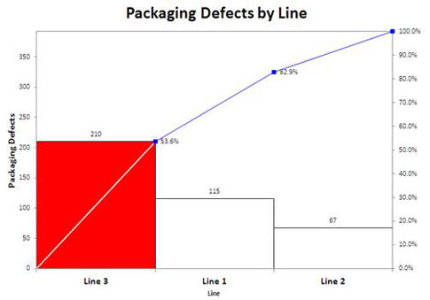
Figure 8: Pareto chart of packaging defects by the production lines 1, 2, and 3

Drill down

Production line 3 accounts for 53.6 percent of all packaging defects. However, you should never stop with just one look at the data. Production line 3 is the largest contributor of defects, but drill down to find out more. How do you do it?

Tip: Double-click on any cell in a PivotTable to bring up the data behind it, as shown in figure 9.

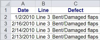
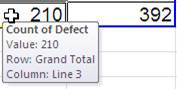
Figure 9: Example of data revealed by clicking on a cell for production line 3

Double-clicking on the Grand Total for production line 3 brings up the data for just line 3. Then pivot column C (the type of defects) and draw a Pareto chart from the resulting summary (see figure 10).

Figure 10: Pareto chart of the type of packaging defects from production line 3

So, folded flaps accounted for 39.5 percent of packaging defects on production line 3. Narrowing the focus makes it easy to write a problem statement for the fishbone diagram (see figure 11) and to convene the right people to analyze the problem.

Figure 11: A fishbone diagram helps visualize data in an organized manner to propose a solution for the defect stated in the problem statement.

Look for additional improvement projects

More than half of the packaging defects occurred on production line 3, but what about lines 1 and 2?

Tip: Use drag and drop to find interesting Pareto patterns in the data.

To find more improvement projects, we could remove the dates from the left column of the original PivotTable and drag in the defects (see figure 12) to show defects by production line.

Figure 12: Drag and drop fields to organize data differently and find other areas in need of improvement

Then run Pareto charts on defects by production line 1 (figure 13) and production line 2 (figure 14).

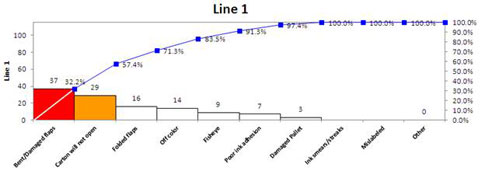
Figure 13: Pareto chart of the type of packaging defects from production line 1

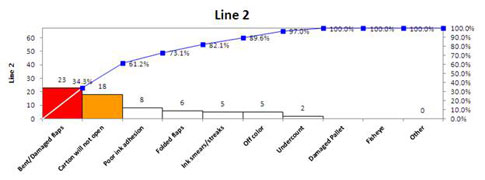
Figure 14: Pareto chart of the type of packaging defects from production line 2

Production lines 1 and 2 have similar issues. Line 1 could do root cause analysis on “Bent/damaged flaps,” while line 2 could work on “Carton will not open.” Solutions from each of the three production lines could be replicated to the other lines to maximize defect reduction across all three lines.

Hidden low-hanging fruit

Most people talk about the “low-hanging fruit” available with Six Sigma, but I have found that it’s often “hidden” in spreadsheets such as these. It requires some data mining with Excel PivotTables and some control charts and Pareto charts to narrow the focus to find the hidden low-hanging fruit. Then it’s easy to get the right people together to diagnose the cause and implement countermeasures.

Tip: There’s usually more than one improvement project in these kinds of data sets, so dramatic improvements are possible by having multiple teams work on multiple “big bars.”